Fisher's exact test failure can lead to biased results

Robersy Sanchez

Department of Biology. Pennsylvania State University, University Park, PA 16802

Email: rus547@psu.edu

Fisher’s exact test is a statistical significance test used in the analysis of contingency tables. Although this test is routinely used even though, it has been full of with controversy for over 80 years. Herein, the case of its application analyzed is scrutinized with specific examples.

Overwiew

The statistical significance of the difference between two bisulfite sequence from control and treatment groups at each CG site can be evaluated with Fisher’s exact test. This is a statistical test used to determine if there are nonrandom associations between two categorical variables.

Let there exist two such (categorical) variables $X$ and $Y$, where $X$ stands for two groups of individuals: control and treatment, and $Y$ be a two states variable denoting the methylation status, carrying the number of times that a cytosine site is found methylated ($^{m}CG$) and non-methylated ($CG$), respectively.

This information can be summarized in a $2 \times 2$ table, a $2 \times 2$ matrix in which the entries $a_{ij}$ represent the number of observations in which $x=i$ and $y=j$. Calculate the row and column sums $R_i$ and $C_j$, respectively, and the total sum:

$N=\sum_iR_i=\sum_jC_j$

of the matrix:

  $Y = ^mCG$ $Y = CG$ $R_i$
Control $a_{11}$ $a_12$ $a_{11}+a_{12}$
Treatment $a_{21}$ $a_22$ $a_{21}+a_{22}$
$C_i$ $a_{11}+a_{21}$ $a_{12}+a_{22}$ $a_{11}+a_{12}+a_{21}+a_{22} = N$

Then the conditional probability of getting the actual matrix, given the particular row and column sums, is given by the formula:

$P_{cutoff}=\frac{R_1!R_2!}{N!\prod_{i,j}a_{ij}!}C_1!C_2!$

A Short Introduction to Algebraic Taxonomy on Genes Regions

a-short-introduction-to-algebraic-taxonomy-on-genes-regions

Optimal cutpoint for the methylation signal

Detection of the methylation signal with Methyl-IT


The discrimination of the methylation signal from the stochastic methylation background resultant from the standard (non-stressful) biological processes is a critical step for the genome-wide methylation analysis. Such a discrimination requires for the knowledge of the probability distribution of the information divergence of methylation levels and a proper evaluation of the classification performance of differentially methylated positions (DMPs) into two classes: DMPs from control and DMPs from treatment.

Background


The probability of extreme methylation changes occurring spontaneously in a control population by the stochastic fluctuations inherent to biochemical processes and DNA maintenance (1), requires the discrimination of this background variation from a biological treatment signal. The stochasticity of the the methylation process derives from the stochasticity inherent to biochemical processes (2-3). There are fundamental physical reasons to acknowledge that biochemical processes are subject to noise and fluctuations (4-5). So, regardless constant environment, statistically significant methylation changes can be found in control population with probability greater than zero and proportional to a Boltzmann factor (6).

Natural signals and those generated by human technology are not free of noise and, as mentioned above, the methylation signal is no exception. Only signal detection based approaches are designed to filter out the signal from the noise, in natural and in human generated signals.

The stochasticity of methylation regulatory machinery effects is presumed to reflect system heterogeneity; cells from the same tissue are not necessarily in the same state, and therefore, corresponding cytosine sites differ in their methylation status. Consequently, overall organismal response is conveyed as a statistical outcome that distinguishes the regulatory methylation signal from statistical background “noise”. Estimation of optimal cutoff value for the signal is an additional step to remove any remaining potential methylation background noise with probability $0 ≤ \alpha ≤ 0.05$. We define as a methylation signal (DMP) each cytosine site with Hellinger Divergence values above the cutpoint (shown in (7)).

As a result, a differentially methylated position (DMP) as a cytosine position with high probability to be altered in methylation due to a treatment effect, distinct from spontaneous variation detected in the control population.

Note: This example was made with the MethylIT version 0.3.2 available at https://github.com/genomaths/MethylIT.
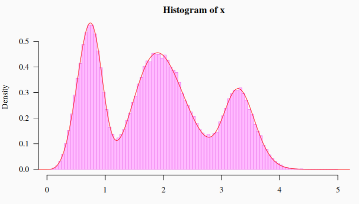
Data generation


For the current example on methylation analysis with Methyl-IT we will use simulated data. Read-count matrices of methylated and unmethylated cytosine are generated with MethylIT.utils function simulateCounts. A standard analysis of this dataset is given in the web page: Methylation analysis with Methyl-IT

library(MethylIT)
library(MethylIT.utils)

bmean <- function(alpha, beta) alpha/(alpha + beta)
alpha.ct <- 0.09
alpha.tt <- 0.2

# The number of cytosine sites to generate
sites = 50000 
# Set a seed for pseudo-random number generation
set.seed(124)
control.nam <- c("C1", "C2", "C3")
treatment.nam <- c("T1", "T2", "T3")

# Reference group 
ref0 = simulateCounts(num.samples = 4, sites = sites, alpha = alpha.ct, beta = 0.5,
                      size = 50, theta = 4.5, sample.ids = c("R1", "R2", "R3", "R4"))
# Control group
ctrl = simulateCounts(num.samples = 3, sites = sites, alpha = alpha.ct, beta = 0.5,
                      size = 50, theta = 4.5, sample.ids = control.nam)
# Treatment group
treat = simulateCounts(num.samples = 3, sites = sites, alpha = alpha.tt, beta = 0.5,
                       size = 50, theta = 4.5, sample.ids = treatment.nam)

# Reference sample
ref = poolFromGRlist(ref0, stat = "mean", num.cores = 4L, verbose = FALSE)

Methylation level divergences


Total variation distance and Hellinger divergence are computed with estimateDivergence function

divs <- estimateDivergence(ref = ref, indiv = c(ctrl, treat), Bayesian = TRUE, 
                           num.cores = 6L, percentile = 1, verbose = FALSE)

To get some statistical description about the sample is useful. Here, empirical critical values for the probability distribution of $H$ and $TV$ can is obtained using quantile function from the R package stats.

critical.val <- do.call(rbind, lapply(divs, function(x) {
  x <- x[x$hdiv > 0]
  hd.95 = quantile(x$hdiv, 0.95)
  tv.95 = quantile(abs(x$TV), 0.95)
  return(c(tv = tv.95, hd = hd.95))
}))
critical.val
##       tv.95%    hd.95%
## C1 0.6842105  66.76081
## C2 0.6800000  66.71995
## C3 0.6777456  65.98495
## T1 0.9397681 138.68237
## T2 0.9478351 141.72637
## T3 0.9466565 141.77241

Estimation of potential DMPs with Methyl-IT


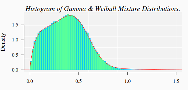
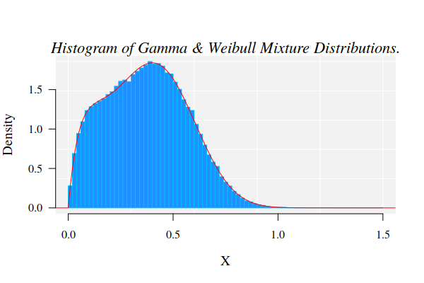
In Methyl-IT, DMP estimation requires for the knowledge of the probability distribution of the noise (plus signal), which is used as null hypothesis.

The best fitted distribution model can be estimated with function gofReport. Here, for illustration purposes, we will use specific estimations based on 2- and 3-parameter gamma distribution models directly using function nonlinearFitDist.

Potential DMPs estimated with 2-parameter gamma distribution model

nlms.g2p <- nonlinearFitDist(divs, column = 9L, verbose = FALSE, num.cores = 6L,
                            dist.name = "Gamma2P")

# Potential DMPs from 'Gamma2P' model
pDMPs.g2p <- getPotentialDIMP(LR = divs, nlms = nlms.g2p,  div.col = 9L, 
                             tv.cut = 0.68, tv.col = 7, alpha = 0.05, 
                             dist.name = "Gamma2P")

Potential DMPs estimated with 3-parameter gamma distribution model

nlms.g3p <- nonlinearFitDist(divs, column = 9L, verbose = FALSE, num.cores = 6L,
                            dist.name = "Gamma3P")

# Potential DMPs from 'Gamma2P' model
pDMPs.g3p <- getPotentialDIMP(LR = divs, nlms = nlms.g3p,  div.col = 9L, 
                             tv.cut = 0.68, tv.col = 7, alpha = 0.05, 
                             dist.name = "Gamma3P")

Cutpoint estimation


As a result of the natural spontaneous variation, naturally occurring DMPs can be identified in samples from the control and treatment populations. Machine-learning algorithms implemented in Methyl-IT are applied to discriminate treatment-induced DMPs from those naturally generated.

The simple cutpoint estimation available in Methyl-IT is based on the application of Youden index (8). Although cutpoints are estimated for a single variable, the classification performance can be evaluated for several variables and applying different model classifiers.

In the current example, the column carrying TV (div.col = 7L) will be used to estimate the cutpoint. The column values will be expressed in terms of $TV_d=|p_{tt}-p_{ct}|$. A minimum cutpoint value for TV derived from the minimum 95% quantile (tv.cut = 0.92) found in the treatment group will be applied (see Methylation analysis with Methyl-IT).

Next, a logistic model classifier will be fitted with the 60% (prop = 0.6) of the raw data (training set) and then the resting 40% of individual samples will be used to evaluate the model performance. The predictor variable included in the model are specified with function parameter column (for more detail see estimateCutPoint or type ?estimateCutPoint in R console).

Simple cutpoint estimation for Gamma2P model

Here, we use the results of modeling the distribution of the Hellinger divergence (HD) of methylation levels through a 2-parameter gamma probability distribution model. The critical values for $HD_{\alpha = 0.05}^{CT_{G2P}}$ used to get potential DMPs were:

nams <- names(nlms.g2p)
crit <- unlist(lapply(nlms.g2p, function(x) qgamma(0.95, shape = x$Estimate[1],
                                                   scale = x$Estimate[2])))
names(crit) <- nams
crit
##        C1        C2        C3        T1        T2        T3 
##  58.59180  57.99972  57.81016 112.40001 113.92362 114.48802

As before the cutpoint is estimated based on 'Youden Index' (8). A PCA+LDA model classifier (classifier = "pca.lda") is applied. That is, a principal component analysis (PCA) is applied on the original raw matrix of data and the four possible component (n.pc = 4) derived from the analysis are used in a further linear discriminant analysis (LDA). A scaling step is applied to the raw matrix of data before the application of the mentioned procedure (center = TRUE, scale = TRUE). Here, PCA will yield new orthogonal (non-correlated) variables, the principal components, which prevent any potential bias effect originated by any correlation or association of the original variables.

By using function estimateCutPoint, we can estimate the cutpoint, based on HD (div.col = 9L) or on $TV_d$ (div.col = 7L):

# Cutpoint estimation for the FT approach using the ECDF critical value
cut.g2p = estimateCutPoint(LR = pDMPs.g2p, simple = TRUE,
                            column = c(hdiv = TRUE, bay.TV = TRUE, 
                                       wprob = TRUE, pos = TRUE),
                            classifier1 = "pca.lda", n.pc = 4, 
                            control.names = control.nam,
                            treatment.names = treatment.nam,
                            center = TRUE, scale = TRUE,
                            clas.perf = TRUE, prop = 0.6,
                           div.col = 9L)
cut.g2p
## Cutpoint estimation with 'Youden Index' 
## Simple cutpoint estimation 
## Cutpoint = 114.22 
## 
## Cytosine sites from treatment have divergence values >= 114.22 
## 
## The accessible objects in the output list are: 
##                     Length Class           Mode     
## cutpoint            1      -none-          numeric  
## testSetPerformance  6      confusionMatrix list     
## testSetModel.FDR    1      -none-          numeric  
## model               2      pcaLDA          list     
## modelConfMatrix     6      confusionMatrix list     
## initModel           1      -none-          character
## postProbCut         1      -none-          logical  
## postCut             1      -none-          logical  
## classifier          1      -none-          character
## statistic           1      -none-          logical  
## optStatVal          1      -none-          logical  
## cutpData            1      -none-          logical  
## initModelConfMatrix 6      confusionMatrix list

As indicated above, the model classifier performance and its corresponding false discovery rate can be retrieved as:

cut.g2p$testSetPerformance
## Confusion Matrix and Statistics
## 
##           Reference
## Prediction   CT   TT
##         CT  319    0
##         TT    0 3544
##                                     
##                Accuracy : 1         
##                  95% CI : (0.999, 1)
##     No Information Rate : 0.9174    
##     P-Value [Acc > NIR] : < 2.2e-16 
##                                     
##                   Kappa : 1         
##                                     
##  Mcnemar's Test P-Value : NA        
##                                     
##             Sensitivity : 1.0000    
##             Specificity : 1.0000    
##          Pos Pred Value : 1.0000    
##          Neg Pred Value : 1.0000    
##              Prevalence : 0.9174    
##          Detection Rate : 0.9174    
##    Detection Prevalence : 0.9174    
##       Balanced Accuracy : 1.0000    
##                                     
##        'Positive' Class : TT        
## 
cut.g2p$testSetModel.FDR
## [1] 0

Here, DMP classification is modeled with PCA+QDA classifier (classifier = "pca.lda"). That is, principal component analysis (PCA) is applied on the original raw matrix of data and the four possible component (n.pc = 4) are used in a further linear discriminant analysis (LDA). A scaling step is applied to the raw matrix of data before the application of the mentioned procedure (center = TRUE, scale = TRUE). Next, a different model classifier can be applied to model the classification derived from the previous cutpoint estimation.

Simple cutpoint estimation for Gamma3P model

The same analyses for the cutpoint estimation can be performed for 3P gamma model

# Cutpoint estimation for the FT approach using the ECDF critical value
cut.g3p = estimateCutPoint(LR = pDMPs.g3p, simple = TRUE,
                            column = c(hdiv = TRUE, bay.TV = TRUE, 
                                       wprob = TRUE, pos = TRUE),
                            classifier1 = "pca.lda", n.pc = 4, 
                            control.names = control.nam,
                            treatment.names = treatment.nam,
                            center = TRUE, scale = TRUE,
                            clas.perf = TRUE, prop = 0.6,
                           div.col = 9L)
cut.g3p
## Cutpoint estimation with 'Youden Index' 
## Simple cutpoint estimation 
## Cutpoint = 115.24 
## 
## Cytosine sites from treatment have divergence values >= 115.24 
## 
## The accessible objects in the output list are: 
##                     Length Class           Mode     
## cutpoint            1      -none-          numeric  
## testSetPerformance  6      confusionMatrix list     
## testSetModel.FDR    1      -none-          numeric  
## model               2      pcaLDA          list     
## modelConfMatrix     6      confusionMatrix list     
## initModel           1      -none-          character
## postProbCut         1      -none-          logical  
## postCut             1      -none-          logical  
## classifier          1      -none-          character
## statistic           1      -none-          logical  
## optStatVal          1      -none-          logical  
## cutpData            1      -none-          logical  
## initModelConfMatrix 6      confusionMatrix list

As indicated above, the model classifier performance and its corresponding false discovery rate can be retrieved as:

cut.g3p$testSetPerformance
## Confusion Matrix and Statistics
## 
##           Reference
## Prediction   CT   TT
##         CT  309    0
##         TT    0 3483
##                                     
##                Accuracy : 1         
##                  95% CI : (0.999, 1)
##     No Information Rate : 0.9185    
##     P-Value [Acc > NIR] : < 2.2e-16 
##                                     
##                   Kappa : 1         
##                                     
##  Mcnemar's Test P-Value : NA        
##                                     
##             Sensitivity : 1.0000    
##             Specificity : 1.0000    
##          Pos Pred Value : 1.0000    
##          Neg Pred Value : 1.0000    
##              Prevalence : 0.9185    
##          Detection Rate : 0.9185    
##    Detection Prevalence : 0.9185    
##       Balanced Accuracy : 1.0000    
##                                     
##        'Positive' Class : TT        
## 
cut.g3p$testSetModel.FDR
## [1] 0

DMP prediction based on classification models

The model obtained in the previous step can be used for further prediction with function predict from MethylIT.utils package. For example, we would take a random sample and run:

set.seed(1)
randsampl <- unlist(pDMPs.g3p)
randsampl <- randsampl[sample.int(length(randsampl), 10)]

pred <- predict(cut.g3p$model, newdata = randsampl)
pred
## $class
##  [1] CT TT TT TT TT TT TT TT TT TT
## Levels: CT TT
## 
## $posterior
##                 CT          TT
##  [1,] 1.000000e+00 1.19242e-08
##  [2,] 5.231187e-46 1.00000e+00
##  [3,] 2.136182e-45 1.00000e+00
##  [4,] 6.739051e-47 1.00000e+00
##  [5,] 2.015394e-46 1.00000e+00
##  [6,] 2.379968e-46 1.00000e+00
##  [7,] 3.473689e-46 1.00000e+00
##  [8,] 1.760048e-46 1.00000e+00
##  [9,] 7.640639e-47 1.00000e+00
## [10,] 3.254017e-47 1.00000e+00
## 
## $x
##             LD1
##  [1,] -7.465499
##  [2,]  1.041471
##  [3,]  0.943772
##  [4,]  1.183774
##  [5,]  1.107704
##  [6,]  1.096158
##  [7,]  1.069901
##  [8,]  1.117111
##  [9,]  1.175055
## [10,]  1.234328

The variable pred$posterior provides the posterior classification probabilities that a DMP could belong to control (CT) or to treatment (TT) group. The variable 'x' provides the cytosine methylation changes in terms of its values in the linear discriminant function LD1. Notice that, for each row, the sum of posterior probabilities is equal 1. By default, individuals with TT posterior probabilities greater than 0.5 are predicted to belong to the treatment class. For example:

classfiction = rep("CT", 10)
classfiction[pred$posterior[, 2] > 0.5] <- "TT"
classfiction
##  [1] "CT" "TT" "TT" "TT" "TT" "TT" "TT" "TT" "TT" "TT"

We can be more strict increasing the posterior classification probability cutoff

classfiction = rep("CT", 10)
classfiction[pred$posterior[, 2] > 0.7] <- "TT"
classfiction
##  [1] "CT" "TT" "TT" "TT" "TT" "TT" "TT" "TT" "TT" "TT"

The posterior classification probability cutoff can be controlled with parameter post.cut from estimateCutPoint function (default: $post.cut=0.5$).

Machine-learning (ML) based approach to search for an optimal cutpoint


In the next example the cutpoint estimation for the Hellinger divergence of methylation levels (div.col = 9L) is accomplished. Function estimateCutPoint can be used to search for a cutpoint as well. Two model classifiers can be used. classifiers1 will be used to estimate the posterior classification probabilities of DMP into those from control and those from treatment. These probabilities are then used to estimate the cutpoint in the range of values from, say, 0.5 to 0.8. Next, a classifier2 will be used to evaluate the classification performance. In this case, the search for an optimal cutpoint is accomplished maximizing the accuracy (stat = 0) of classifier2.

ML cutpoint estimation for potential DMPs based on Gamma2P model

The ML search for an optimal cutpoint is accomplished in the set of potential DMPs, which were identified using a Gamma2P probability distribution model as null hypothesis.

cut.g2p = estimateCutPoint(LR = pDMPs.g2p, simple = FALSE,
                            column = c(hdiv = TRUE, bay.TV = TRUE, 
                                       wprob = TRUE, pos = TRUE),
                            classifier1 = "pca.lda", 
                            classifier2 = "pca.qda", stat = 0,
                            control.names = control.nam, 
                            treatment.names = treatment.nam, 
                            cut.values = seq(45, 114, 1), post.cut = 0.5,
                            clas.perf = TRUE, prop = 0.6,
                            center = TRUE, scale = TRUE,
                            n.pc = 4, div.col = 9L)
cut.g2p
## Cutpoint estimation with 'pca.lda' classifier 
## Cutpoint search performed using model posterior probabilities 
## 
## Posterior probability used to get the cutpoint = 0.5 
## Cytosine sites with treatment PostProbCut >= 0.5 have a 
## divergence value >= 112.4247 
## 
## Optimized statistic: Accuracy = 1 
## Cutpoint = 112.42 
## 
## Model classifier 'pca.qda' 
## 
## The accessible objects in the output list are: 
##                    Length Class           Mode     
## cutpoint           1      -none-          numeric  
## testSetPerformance 6      confusionMatrix list     
## testSetModel.FDR   1      -none-          numeric  
## model              2      pcaQDA          list     
## modelConfMatrix    6      confusionMatrix list     
## initModel          1      -none-          character
## postProbCut        1      -none-          numeric  
## postCut            1      -none-          numeric  
## classifier         1      -none-          character
## statistic          1      -none-          character
## optStatVal         1      -none-          numeric  
## cutpData           1      -none-          logical

Model performance in the test dataset is:

cut.g2p$testSetPerformance
## Confusion Matrix and Statistics
## 
##           Reference
## Prediction   CT   TT
##         CT 1274    0
##         TT    0 3580
##                                      
##                Accuracy : 1          
##                  95% CI : (0.9992, 1)
##     No Information Rate : 0.7375     
##     P-Value [Acc > NIR] : < 2.2e-16  
##                                      
##                   Kappa : 1          
##                                      
##  Mcnemar's Test P-Value : NA         
##                                      
##             Sensitivity : 1.0000     
##             Specificity : 1.0000     
##          Pos Pred Value : 1.0000     
##          Neg Pred Value : 1.0000     
##              Prevalence : 0.7375     
##          Detection Rate : 0.7375     
##    Detection Prevalence : 0.7375     
##       Balanced Accuracy : 1.0000     
##                                      
##        'Positive' Class : TT         
## 

Model performance in in the whole dataset is:

cut.g2p$modelConfMatrix
## Confusion Matrix and Statistics
## 
##           Reference
## Prediction   CT   TT
##         CT 3184    0
##         TT    0 8948
##                                      
##                Accuracy : 1          
##                  95% CI : (0.9997, 1)
##     No Information Rate : 0.7376     
##     P-Value [Acc > NIR] : < 2.2e-16  
##                                      
##                   Kappa : 1          
##                                      
##  Mcnemar's Test P-Value : NA         
##                                      
##             Sensitivity : 1.0000     
##             Specificity : 1.0000     
##          Pos Pred Value : 1.0000     
##          Neg Pred Value : 1.0000     
##              Prevalence : 0.7376     
##          Detection Rate : 0.7376     
##    Detection Prevalence : 0.7376     
##       Balanced Accuracy : 1.0000     
##                                      
##        'Positive' Class : TT         
## 

The False discovery rate is:

cut.g2p$testSetModel.FDR
## [1] 0

The model classifier PCA+LDA has enough discriminatory power to discriminate control DMP from those induced by the treatment for HD values $112.4247 \le HD$.

The probabilities $P(HD \le 122.43)$ to observe a cytosine site with $HD \le 112.4247$ on each individual is:

nams <- names(nlms.g2p)
crit <- unlist(lapply(nlms.g2p, function(x) pgamma(cut.g2p$cutpoint, shape = x$Estimate[1],
                                                   scale = x$Estimate[2])))
names(crit) <- nams
crit
##        C1        C2        C3        T1        T2        T3 
## 0.9964704 0.9966560 0.9967314 0.9500279 0.9483024 0.9476610

In other words, most of the methylation changes are not (and should not be) considered DMPs. Notice that although the same HD value could be found in the same differentially methylated cytosine site in control and treatment, if the probabilities distributions of the information divergences (null hypotheses) from control and treatment are different, then these DMPs can be distinguished.

ML cutpoint estimation for potential DMPs based on Gamma3P model

Likewise, for the 3-parameter gamma model we can search for an optimal cutpoint:

cut.g3p = estimateCutPoint(LR = pDMPs.g3p, simple = FALSE,
                            column = c(hdiv = TRUE, TV = TRUE, 
                                       wprob = TRUE, pos = TRUE),
                            classifier1 = "pca.lda", 
                            classifier2 = "pca.qda", stat = 0,
                            control.names = control.nam, 
                            treatment.names = treatment.nam, 
                            cut.values = seq(45, 114, 1), post.cut = 0.5,
                            clas.perf = TRUE, prop = 0.6,
                            center = TRUE, scale = TRUE,
                            n.pc = 4, div.col = 9L)
cut.g3p
## Cutpoint estimation with 'pca.lda' classifier 
## Cutpoint search performed using model posterior probabilities 
## 
## Posterior probability used to get the cutpoint = 0.5 
## Cytosine sites with treatment PostProbCut >= 0.5 have a 
## divergence value >= 113.497 
## 
## Optimized statistic: Accuracy = 1 
## Cutpoint = 113.5 
## 
## Model classifier 'pca.qda' 
## 
## The accessible objects in the output list are: 
##                    Length Class           Mode     
## cutpoint           1      -none-          numeric  
## testSetPerformance 6      confusionMatrix list     
## testSetModel.FDR   1      -none-          numeric  
## model              2      pcaQDA          list     
## modelConfMatrix    6      confusionMatrix list     
## initModel          1      -none-          character
## postProbCut        1      -none-          numeric  
## postCut            1      -none-          numeric  
## classifier         1      -none-          character
## statistic          1      -none-          character
## optStatVal         1      -none-          numeric  
## cutpData           1      -none-          logical

DMPs are identified with function selectDIMP

g2p.dmps <- selectDIMP(pDMPs.g2p, div.col = 9L, cutpoint = cut.g2p$cutpoint)
g3p.dmps <- selectDIMP(pDMPs.g3p, div.col = 9L, cutpoint = cut.g3p$cutpoint)

DMPs estimated with Fisher's exact Test (FT)

For comparison purposes DMPs are estimated with Fisher's exact test as well.

ft. = FisherTest(LR = divs, tv.cut = 0.68, pAdjustMethod = "BH",
                     pvalCutOff = 0.05, num.cores = 4L,
                     verbose = FALSE, saveAll = FALSE) 

ft.dmps <- getPotentialDIMP(LR = ft., div.col = 9L, dist.name = "None",
                            tv.cut = 0.68, tv.col = 7, alpha = 0.05)

Classification performance of DMP classification


After the cutpoint application to select DMPs, a Monte Carlo (bootstrap) analysis reporting several classifier performance indicators can be accomplished by using function evaluateDIMPclass and its settings output = "mc.val" and num.boot.

Classification performance for DMPs based on Gamma2P model

g2p.class = evaluateDIMPclass(LR = g2p.dmps, control.names = control.nam,
                           treatment.names = treatment.nam,
                           column = c(hdiv = TRUE, TV = TRUE, 
                                      wprob = TRUE, pos = TRUE),
                           classifier = "pca.qda", n.pc = 4, 
                           center = TRUE, scale = TRUE, num.boot = 300,
                           output = "all", prop = 0.6
)
g2p.class$mc.val
##     Accuracy     Kappa   AccuracyLower    AccuracyUpper  AccuracyNull   
##  Min.   :1   Min.   :1   Min.   :0.9991   Min.   :1     Min.   :0.9139  
##  1st Qu.:1   1st Qu.:1   1st Qu.:0.9991   1st Qu.:1     1st Qu.:0.9139  
##  Median :1   Median :1   Median :0.9991   Median :1     Median :0.9139  
##  Mean   :1   Mean   :1   Mean   :0.9991   Mean   :1     Mean   :0.9139  
##  3rd Qu.:1   3rd Qu.:1   3rd Qu.:0.9991   3rd Qu.:1     3rd Qu.:0.9139  
##  Max.   :1   Max.   :1   Max.   :0.9991   Max.   :1     Max.   :0.9139  
##                                                                         
##  AccuracyPValue       McnemarPValue  Sensitivity  Specificity Pos Pred Value
##  Min.   :9.096e-154   Min.   : NA   Min.   :1    Min.   :1    Min.   :1     
##  1st Qu.:9.096e-154   1st Qu.: NA   1st Qu.:1    1st Qu.:1    1st Qu.:1     
##  Median :9.096e-154   Median : NA   Median :1    Median :1    Median :1     
##  Mean   :9.096e-154   Mean   :NaN   Mean   :1    Mean   :1    Mean   :1     
##  3rd Qu.:9.096e-154   3rd Qu.: NA   3rd Qu.:1    3rd Qu.:1    3rd Qu.:1     
##  Max.   :9.096e-154   Max.   : NA   Max.   :1    Max.   :1    Max.   :1     
##                       NA's   :300                                           
##  Neg Pred Value   Precision     Recall        F1      Prevalence    
##  Min.   :1      Min.   :1   Min.   :1   Min.   :1   Min.   :0.9139  
##  1st Qu.:1      1st Qu.:1   1st Qu.:1   1st Qu.:1   1st Qu.:0.9139  
##  Median :1      Median :1   Median :1   Median :1   Median :0.9139  
##  Mean   :1      Mean   :1   Mean   :1   Mean   :1   Mean   :0.9139  
##  3rd Qu.:1      3rd Qu.:1   3rd Qu.:1   3rd Qu.:1   3rd Qu.:0.9139  
##  Max.   :1      Max.   :1   Max.   :1   Max.   :1   Max.   :0.9139  
##                                                                     
##  Detection Rate   Detection Prevalence Balanced Accuracy
##  Min.   :0.9139   Min.   :0.9139       Min.   :1        
##  1st Qu.:0.9139   1st Qu.:0.9139       1st Qu.:1        
##  Median :0.9139   Median :0.9139       Median :1        
##  Mean   :0.9139   Mean   :0.9139       Mean   :1        
##  3rd Qu.:0.9139   3rd Qu.:0.9139       3rd Qu.:1        
##  Max.   :0.9139   Max.   :0.9139       Max.   :1        
## 

Classification performance for DMPs based on Gamma3P model

Likewise the evaluation of the DMP classification performance can be accomplished for DMPs estimated based on the $'Gamma3P'$ model:

g3p.class = evaluateDIMPclass(LR = g3p.dmps, control.names = control.nam,
                           treatment.names = treatment.nam,
                           column = c(hdiv = TRUE, TV = TRUE, 
                                      wprob = TRUE, pos = TRUE),
                           classifier = "pca.qda", n.pc = 4, 
                           center = TRUE, scale = TRUE, num.boot = 300,
                           output = "all", prop = 0.6
)
g3p.class$mc.val
##     Accuracy     Kappa   AccuracyLower   AccuracyUpper  AccuracyNull  
##  Min.   :1   Min.   :1   Min.   :0.999   Min.   :1     Min.   :0.914  
##  1st Qu.:1   1st Qu.:1   1st Qu.:0.999   1st Qu.:1     1st Qu.:0.914  
##  Median :1   Median :1   Median :0.999   Median :1     Median :0.914  
##  Mean   :1   Mean   :1   Mean   :0.999   Mean   :1     Mean   :0.914  
##  3rd Qu.:1   3rd Qu.:1   3rd Qu.:0.999   3rd Qu.:1     3rd Qu.:0.914  
##  Max.   :1   Max.   :1   Max.   :0.999   Max.   :1     Max.   :0.914  
##                                                                       
##  AccuracyPValue       McnemarPValue  Sensitivity  Specificity Pos Pred Value
##  Min.   :1.393e-150   Min.   : NA   Min.   :1    Min.   :1    Min.   :1     
##  1st Qu.:1.393e-150   1st Qu.: NA   1st Qu.:1    1st Qu.:1    1st Qu.:1     
##  Median :1.393e-150   Median : NA   Median :1    Median :1    Median :1     
##  Mean   :1.393e-150   Mean   :NaN   Mean   :1    Mean   :1    Mean   :1     
##  3rd Qu.:1.393e-150   3rd Qu.: NA   3rd Qu.:1    3rd Qu.:1    3rd Qu.:1     
##  Max.   :1.393e-150   Max.   : NA   Max.   :1    Max.   :1    Max.   :1     
##                       NA's   :300                                           
##  Neg Pred Value   Precision     Recall        F1      Prevalence   
##  Min.   :1      Min.   :1   Min.   :1   Min.   :1   Min.   :0.914  
##  1st Qu.:1      1st Qu.:1   1st Qu.:1   1st Qu.:1   1st Qu.:0.914  
##  Median :1      Median :1   Median :1   Median :1   Median :0.914  
##  Mean   :1      Mean   :1   Mean   :1   Mean   :1   Mean   :0.914  
##  3rd Qu.:1      3rd Qu.:1   3rd Qu.:1   3rd Qu.:1   3rd Qu.:0.914  
##  Max.   :1      Max.   :1   Max.   :1   Max.   :1   Max.   :0.914  
##                                                                    
##  Detection Rate  Detection Prevalence Balanced Accuracy
##  Min.   :0.914   Min.   :0.914        Min.   :1        
##  1st Qu.:0.914   1st Qu.:0.914        1st Qu.:1        
##  Median :0.914   Median :0.914        Median :1        
##  Mean   :0.914   Mean   :0.914        Mean   :1        
##  3rd Qu.:0.914   3rd Qu.:0.914        3rd Qu.:1        
##  Max.   :0.914   Max.   :0.914        Max.   :1        
## 

We do not have evidence to support statistical differences between the classification performances estimated for 'Gamma2P' and 'Gamma3P' probability distribution models. Hence, in this case we select the model that yield the lowest cutpoint

Classification performance for DMPs based on Fisher's exact test

Classification performance results obtained with Monte Carlos sampling for the $Gamma2P$ and $Gamma3P$ models are quite different from those obtained with FT:

ft.class = evaluateDIMPclass(LR = ft.dmps, control.names = control.nam,
                           treatment.names = treatment.nam, 
                           column = c(hdiv = TRUE, TV = TRUE, 
                                      wprob = TRUE, pos = TRUE),
                           classifier = "pca.lda", n.pc = 4, 
                           center = TRUE, scale = TRUE, num.boot = 300,
                           output = "all", prop = 0.6
)
ft.class$mc.val
##     Accuracy          Kappa           AccuracyLower    AccuracyUpper   
##  Min.   :0.8076   Min.   :-0.007635   Min.   :0.8001   Min.   :0.8148  
##  1st Qu.:0.8105   1st Qu.: 0.005355   1st Qu.:0.8031   1st Qu.:0.8177  
##  Median :0.8110   Median : 0.007678   Median :0.8036   Median :0.8182  
##  Mean   :0.8110   Mean   : 0.007553   Mean   :0.8036   Mean   :0.8182  
##  3rd Qu.:0.8115   3rd Qu.: 0.009748   3rd Qu.:0.8041   3rd Qu.:0.8187  
##  Max.   :0.8137   Max.   : 0.020669   Max.   :0.8064   Max.   :0.8209  
##   AccuracyNull    AccuracyPValue   McnemarPValue  Sensitivity    
##  Min.   :0.8188   Min.   :0.9205   Min.   :0     Min.   :0.9835  
##  1st Qu.:0.8188   1st Qu.:0.9781   1st Qu.:0     1st Qu.:0.9857  
##  Median :0.8188   Median :0.9847   Median :0     Median :0.9863  
##  Mean   :0.8188   Mean   :0.9827   Mean   :0     Mean   :0.9863  
##  3rd Qu.:0.8188   3rd Qu.:0.9888   3rd Qu.:0     3rd Qu.:0.9868  
##  Max.   :0.8188   Max.   :0.9990   Max.   :0     Max.   :0.9893  
##   Specificity      Pos Pred Value   Neg Pred Value     Precision     
##  Min.   :0.01134   Min.   :0.8181   Min.   :0.1337   Min.   :0.8181  
##  1st Qu.:0.01726   1st Qu.:0.8193   1st Qu.:0.2150   1st Qu.:0.8193  
##  Median :0.01874   Median :0.8196   Median :0.2318   Median :0.8196  
##  Mean   :0.01858   Mean   :0.8196   Mean   :0.2304   Mean   :0.8196  
##  3rd Qu.:0.02022   3rd Qu.:0.8198   3rd Qu.:0.2455   3rd Qu.:0.8198  
##  Max.   :0.02663   Max.   :0.8208   Max.   :0.3187   Max.   :0.8208  
##      Recall             F1           Prevalence     Detection Rate  
##  Min.   :0.9835   Min.   :0.8933   Min.   :0.8188   Min.   :0.8053  
##  1st Qu.:0.9857   1st Qu.:0.8950   1st Qu.:0.8188   1st Qu.:0.8071  
##  Median :0.9863   Median :0.8952   Median :0.8188   Median :0.8076  
##  Mean   :0.9863   Mean   :0.8952   Mean   :0.8188   Mean   :0.8076  
##  3rd Qu.:0.9868   3rd Qu.:0.8955   3rd Qu.:0.8188   3rd Qu.:0.8080  
##  Max.   :0.9893   Max.   :0.8969   Max.   :0.8188   Max.   :0.8101  
##  Detection Prevalence Balanced Accuracy
##  Min.   :0.9825       Min.   :0.4975   
##  1st Qu.:0.9848       1st Qu.:0.5017   
##  Median :0.9853       Median :0.5025   
##  Mean   :0.9854       Mean   :0.5024   
##  3rd Qu.:0.9860       3rd Qu.:0.5031   
##  Max.   :0.9879       Max.   :0.5066

A quite different story is found when information on the probability distribution of noise (null hypothesis) is added to the classifier:

ft.g2p.dmps <- getPotentialDIMP(LR = ft., nlms = nlms.g2p,  div.col = 9L, 
                                tv.cut = 0.68, tv.col = 7, alpha = 0.05, 
                                dist.name = "Gamma2P")

ft.g2p.class = evaluateDIMPclass(LR = ft.g2p.dmps, control.names = control.nam,
                                 treatment.names = treatment.nam,
                                 column = c(hdiv = TRUE, TV = TRUE, 
                                            wprob = TRUE, pos = TRUE),
                                 classifier = "pca.lda", n.pc = 4, 
                                 center = TRUE, scale = TRUE, num.boot = 300,
                                 output = "all", prop = 0.6
)
ft.g2p.class$mc.val
##     Accuracy     Kappa   AccuracyLower    AccuracyUpper  AccuracyNull   
##  Min.   :1   Min.   :1   Min.   :0.9992   Min.   :1     Min.   :0.7375  
##  1st Qu.:1   1st Qu.:1   1st Qu.:0.9992   1st Qu.:1     1st Qu.:0.7375  
##  Median :1   Median :1   Median :0.9992   Median :1     Median :0.7375  
##  Mean   :1   Mean   :1   Mean   :0.9992   Mean   :1     Mean   :0.7375  
##  3rd Qu.:1   3rd Qu.:1   3rd Qu.:0.9992   3rd Qu.:1     3rd Qu.:0.7375  
##  Max.   :1   Max.   :1   Max.   :0.9992   Max.   :1     Max.   :0.7375  
##                                                                         
##  AccuracyPValue McnemarPValue  Sensitivity  Specificity Pos Pred Value
##  Min.   :0      Min.   : NA   Min.   :1    Min.   :1    Min.   :1     
##  1st Qu.:0      1st Qu.: NA   1st Qu.:1    1st Qu.:1    1st Qu.:1     
##  Median :0      Median : NA   Median :1    Median :1    Median :1     
##  Mean   :0      Mean   :NaN   Mean   :1    Mean   :1    Mean   :1     
##  3rd Qu.:0      3rd Qu.: NA   3rd Qu.:1    3rd Qu.:1    3rd Qu.:1     
##  Max.   :0      Max.   : NA   Max.   :1    Max.   :1    Max.   :1     
##                 NA's   :300                                           
##  Neg Pred Value   Precision     Recall        F1      Prevalence    
##  Min.   :1      Min.   :1   Min.   :1   Min.   :1   Min.   :0.7375  
##  1st Qu.:1      1st Qu.:1   1st Qu.:1   1st Qu.:1   1st Qu.:0.7375  
##  Median :1      Median :1   Median :1   Median :1   Median :0.7375  
##  Mean   :1      Mean   :1   Mean   :1   Mean   :1   Mean   :0.7375  
##  3rd Qu.:1      3rd Qu.:1   3rd Qu.:1   3rd Qu.:1   3rd Qu.:0.7375  
##  Max.   :1      Max.   :1   Max.   :1   Max.   :1   Max.   :0.7375  
##                                                                     
##  Detection Rate   Detection Prevalence Balanced Accuracy
##  Min.   :0.7375   Min.   :0.7375       Min.   :1        
##  1st Qu.:0.7375   1st Qu.:0.7375       1st Qu.:1        
##  Median :0.7375   Median :0.7375       Median :1        
##  Mean   :0.7375   Mean   :0.7375       Mean   :1        
##  3rd Qu.:0.7375   3rd Qu.:0.7375       3rd Qu.:1        
##  Max.   :0.7375   Max.   :0.7375       Max.   :1        
## 

Now, we add additional information about the optimal cutpoint

ft.g2p_cutp.dmps <- selectDIMP(ft.g2p.dmps, div.col = 9L, cutpoint = cut.g2p$cutpoint)

ft.g2p_cut.class = evaluateDIMPclass(LR = ft.g2p_cutp.dmps, control.names = control.nam,
                                 treatment.names = treatment.nam,
                                 column = c(hdiv = TRUE, TV = TRUE, 
                                            wprob = TRUE, pos = TRUE),
                                 classifier = "pca.lda", n.pc = 4, 
                                 center = TRUE, scale = TRUE, num.boot = 300,
                                 output = "all", prop = 0.6
)
ft.g2p_cut.class$mc.val
##     Accuracy     Kappa   AccuracyLower    AccuracyUpper  AccuracyNull   
##  Min.   :1   Min.   :1   Min.   :0.9991   Min.   :1     Min.   :0.9139  
##  1st Qu.:1   1st Qu.:1   1st Qu.:0.9991   1st Qu.:1     1st Qu.:0.9139  
##  Median :1   Median :1   Median :0.9991   Median :1     Median :0.9139  
##  Mean   :1   Mean   :1   Mean   :0.9991   Mean   :1     Mean   :0.9139  
##  3rd Qu.:1   3rd Qu.:1   3rd Qu.:0.9991   3rd Qu.:1     3rd Qu.:0.9139  
##  Max.   :1   Max.   :1   Max.   :0.9991   Max.   :1     Max.   :0.9139  
##                                                                         
##  AccuracyPValue       McnemarPValue  Sensitivity  Specificity Pos Pred Value
##  Min.   :9.096e-154   Min.   : NA   Min.   :1    Min.   :1    Min.   :1     
##  1st Qu.:9.096e-154   1st Qu.: NA   1st Qu.:1    1st Qu.:1    1st Qu.:1     
##  Median :9.096e-154   Median : NA   Median :1    Median :1    Median :1     
##  Mean   :9.096e-154   Mean   :NaN   Mean   :1    Mean   :1    Mean   :1     
##  3rd Qu.:9.096e-154   3rd Qu.: NA   3rd Qu.:1    3rd Qu.:1    3rd Qu.:1     
##  Max.   :9.096e-154   Max.   : NA   Max.   :1    Max.   :1    Max.   :1     
##                       NA's   :300                                           
##  Neg Pred Value   Precision     Recall        F1      Prevalence    
##  Min.   :1      Min.   :1   Min.   :1   Min.   :1   Min.   :0.9139  
##  1st Qu.:1      1st Qu.:1   1st Qu.:1   1st Qu.:1   1st Qu.:0.9139  
##  Median :1      Median :1   Median :1   Median :1   Median :0.9139  
##  Mean   :1      Mean   :1   Mean   :1   Mean   :1   Mean   :0.9139  
##  3rd Qu.:1      3rd Qu.:1   3rd Qu.:1   3rd Qu.:1   3rd Qu.:0.9139  
##  Max.   :1      Max.   :1   Max.   :1   Max.   :1   Max.   :0.9139  
##                                                                     
##  Detection Rate   Detection Prevalence Balanced Accuracy
##  Min.   :0.9139   Min.   :0.9139       Min.   :1        
##  1st Qu.:0.9139   1st Qu.:0.9139       1st Qu.:1        
##  Median :0.9139   Median :0.9139       Median :1        
##  Mean   :0.9139   Mean   :0.9139       Mean   :1        
##  3rd Qu.:0.9139   3rd Qu.:0.9139       3rd Qu.:1        
##  Max.   :0.9139   Max.   :0.9139       Max.   :1        
## 

In other words, information on the probability distributions of the natural spontaneous methylation variation in the control and treatment population are essential to discriminate the background noise from the treatment induced signal.

Graphics of DMP classification performance


DMP count data:

dt <- t(rbind(G2P = sapply(g2p.dmps, length),
              G3P = sapply(g3p.dmps, length),
              FT = sapply(ft.dmps, length),
              FT.G2P = sapply(ft.g2p.dmps, length),
              FT.SD = sapply(ft.g2p_cutp.dmps, length)
    ))
dt
##     G2P  G3P   FT FT.G2P FT.SD
## C1  255  251 1730   1055   255
## C2  306  298 1682   1070   306
## C3  281  276 1657   1059   281
## T1 2925 2871 7589   2926  2925
## T2 3032 2965 7646   3032  3032
## T3 2990 2934 7679   2990  2990

The comparison between the approaches FT.G2P and FT.SD (full signal detection on FT output) tells us that only 255, 306, and 281 cytosine sites detected with FT in the control samples C1, C2, and C3, respectively, carry methylation signals comparable (in magnitude) to those signals induced by the treatment.

Classification performance data:

df <- data.frame(method = c("FT", "FT.G2P", "FT.SD", "G2P", "G3P"), 
                 rbind(
                       c(colMeans(ft.class$boots)[c(1, 8:11, 18)], FDR = ft.class$con.mat$FDR),
                       c(colMeans(ft.g2p.class$boots)[c(1, 8:11, 18)], FDR = ft.g2p.class$con.mat$FDR),
                       c(colMeans(ft.g2p_cut.class$boots)[c(1, 8:11, 18)], FDR = ft.g2p_cut.class$con.mat$FDR),
                       c(colMeans(g2p.class$boots)[c(1, 8:11, 18)], FDR = g2p.class$con.mat$FDR),
                       c(colMeans(g3p.class$boots)[c(1, 8:11, 18)], FDR = g3p.class$con.mat$FDR)
                 ))

Graphics:

color <- c("darkgreen", "#147714FF", "#3D9F3DFF", "#66C666FF",  "#90EE90FF")
dt <- data.frame(dt, sample = names(g2p.dmps))

## ------------------------- DMP count graphic ---------------------------------
par(family = "serif", lwd = 0.1, cex = 1, mar = c(2,5,2,2), mfcol = c(1, 2))
barplot(cbind(FT, FT.G2P, FT.SD, G2P, G3P) ~ sample, 
        panel.first={points(0, 0, pch=16, cex=1e6, col="grey95")
          grid(col="white", lty = 1, lwd = 1)},
        data = dt, beside = TRUE,  legend.text = TRUE, las = 1, lwd = 0.05, yaxt = "n",
        cex.names = 1.4, font = 3, xlab = "", col = color,
        args.legend = list(x=10, y=6000, text.font = 2, box.lwd = 0, horiz = FALSE,
                           adj = 0, xjust = 0.65, yjust = 0.8, bty = "n", cex = 1.2,
                           x.intersp = 0.2, inset = -1, ncol = 1, fill = color))
axis(2, hadj = 0.9, las = 2, lwd = 0.4, tck = -0.02, cex.axis = 1.2, font = 2, line = -0.2)
mtext(side = 2, text = "DMP count", line = 3, cex = 1.4, font = 3)

## ------------------ DMP classifiction performance graphic -------------------
color <- c("mediumblue", "#0000FFFF", "#3949F6FF", "#566CF2FF", "#7390EEFF", "#90B3EAFF", "#ADD8E6FF")
labs <- df$method
  
par(family = "serif", lwd = 0.1, cex = 1, mar = c(4,2,2,10))
x <- barplot(cbind(Accuracy, Sensitivity, Specificity, Pos.Pred.Value, Neg.Pred.Value, 
              Balanced.Accuracy, FDR) ~ method, 
        panel.first={points(0, 0, pch=16, cex=1e6, col="grey95")
          grid(col="white", lty = 1, lwd = 1)}, 
        data = df, beside = TRUE,  legend.text = TRUE, las = 1, lwd = 0.1, yaxt = "n",
        cex.names = 1.4, font = 3, xlab = "", col = color, ylim = c(0,1), 
        args.legend = list(x = 52, y = 1., text.font = 2, box.lwd = 0, horiz = FALSE,
                           adj = 0, xjust = 0.65, yjust = 0.8, bty = "n", cex = 1.2,
                           x.intersp = 0.2, inset = -1, ncol = 1, fill = color))
axis(2, hadj = 0.8, las = 2, lwd = 0.4, tck = -0.02, cex.axis = 1.2, font = 2,
     line = -0.4)
mtext(side = 2, text = "Performance value", line = 2, cex = 1.4, font = 3)

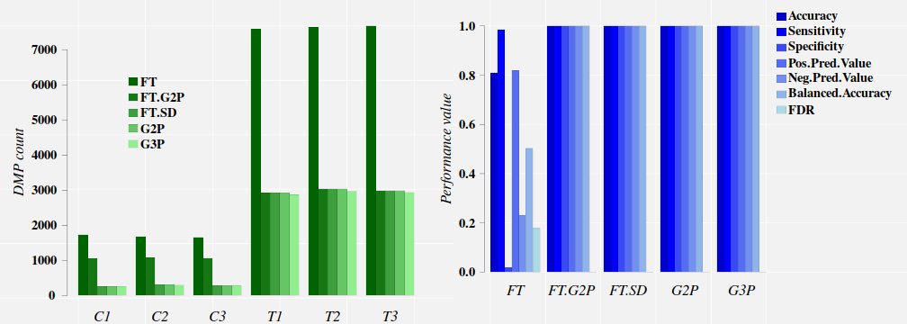
FT.G2P and FT.SD approaches lead to excellent classification performances on this data set. At this point, we can appeal the parsimony principle, follows from Occam’s razor that states “among competing hypotheses, the hypothesis with the fewest assumptions should be selected. In other words, results indicates that the signal-detection and machine-learning approach is sufficient [@ElNaqa2018; @Sanchez2019].

Conclusions


  1. A proper discrimination of the methylation signal from the stochastic methylation background requires for the knowledge of probability distributions of the methylation signal from control and treatment population. Such a knowledge permits a suitable estimation of the cutoff value to discriminate the methylation signal induced by the treatment from the stochastic methylation background detected in the control group.

  2. It does not matter how significant a differentially methylation event for a given cytosine position would be (after the application of some statistical test), but on how big the probability to be observed in the control group is. In simple words, if for a given DMP the probability of to be observed in the control is big enough, then such a DMP did not result from a treatment effect.

  3. A suitable evaluation on how much the mentioned probability can be big enough derives by estimating an optimal cutpoint. But a classification into two groups results from the cutpoint estimation and the problem on the estimation of such a cutpoint is equivalent to find a discriminatory function (as set by Fisher, [@Fisher1938; @Green1979]). Cases with function values below some cutoff are classified in one group, while values above the cutoff are put in the other group.

  4. MethylIT function estimateCutPoint permits the estimation and search for an optimal cutpoint by confronting the problem as in the spirit of the classical signal detection and as a classification problem. The best model classifier will depend on the dataset under study.So, uses must check for which is the model classifier with the best classification performance for his/her dataset.

References


  1. Ngo, Thuy T.M., Jejoong Yoo, Qing Dai, Qiucen Zhang, Chuan He, Aleksei Aksimentiev, and Taekjip Ha. 2016. “Effects of cytosine modifications on DNA flexibility and nucleosome mechanical stability.” Nature Communications 7 (February). Nature Publishing Group: 10813. https://doi.org/10.1038/ncomms10813.

  2. Min, Wei, Liang Jiang, Ji Yu, S C Kou, Hong Qian, and X Sunney Xie. 2005. “Nonequilibrium steady state of a nanometric biochemical system: Determining the thermodynamic driving force from single enzyme turnover time traces.” Nano Letters 5 (12): 2373–8. https://doi.org/10.1021/nl0521773.

  3. Koslover, Elena F, and Andrew J Spakowitz. 2012. “Force fluctuations impact kinetics of biomolecular systems.” Physical Review. E, Statistical, Nonlinear, and Soft Matter Physics 86 (1 Pt 1): 011906. http://www.ncbi.nlm.nih.gov/pubmed/23005451.

  4. Samoilov, Michael S., Gavin Price, and Adam P. Arkin. 2006. “From fluctuations to phenotypes: the physiology of noise.” Science’s STKE : Signal Transduction Knowledge Environment 2006 (366). https://doi.org/10.1126/stke.3662006re17.

  5. Eldar, Avigdor, and Michael B. Elowitz. 2010. “Functional roles for noise in genetic circuits.” Nature Publishing Group. https://doi.org/10.1038/nature09326.

  6. Sanchez, Robersy, and Sally A. Mackenzie. 2016. “Information Thermodynamics of Cytosine DNA Methylation.” Edited by Barbara Bardoni. PLOS ONE 11 (3). Public Library of Science: e0150427. https://doi.org/10.1371/journal.pone.0150427.

  7. Sanchez, Robersy, Xiaodong Yang, Thomas Maher, and Sally Mackenzie. 2019. “Discrimination of DNA Methylation Signal from Background Variation for Clinical Diagnostics.” Int. J. Mol. Sci. 20 (21): 5343. https://doi.org/https://doi.org/10.3390/ijms20215343.

  8. Youden, W. J. 1950. “Index for rating diagnostic tests.” Cancer 3 (1): 32–35. https://doi.org/10.1002/1097-0142(1950)3:1<32::AID-CNCR2820030106>3.0.CO;2-3.

  9. El Naqa, Issam, Dan Ruan, Gilmer Valdes, Andre Dekker, Todd McNutt, Yaorong Ge, Q. Jackie Wu, et al. 2018. “Machine learning and modeling: Data, validation, communication challenges.” Medical Physics 45 (10): e834–e840. https://doi.org/10.1002/mp.12811.

  10. Fisher, R.A. 1938. “The statistical utilization of multiple measurents.” Annals of Eugenics 8: 376–86.

  11. Green, Bert F. 1979. “The Two Kinds of Linear Discriminant Functions and Their Relationship.” Journal of Educational Statistics 4 (3): 247–63.

Non-linear Fit of Mixture Distributions

Fitting Mixture Distributions

1. Background

Mixture Distributions were introduced in a previous postBasically, it is said that a distribution $f(x)$ is a mixture of k components distributions $f_1(x), …, f_k(x)$ if:

$f(x) = \sum_{i=1}^k \pi_i f_i(x)$

where $\pi_i$ are the so called mixing weights, $0 \le \pi_i \le 1$, and $\pi_1 + … + \pi_k = 1$. Here, new data points from distribution will be generated in the standard way: first to pick a distribution, with probabilities given by the mixing weights, and then to generate one observation according to that distribution. More information about mixture distribution can be read in Wikipedia.

Herein, we will show how to fit numerical data to a mixture of probability distributions model.

2. Generating random variables from a mixture of Gamma and Weibull distributions

To generate from a mixture distribution the R package usefr will be used.

library(usefr) 
set.seed(123) # set a seed for random generation
# ========= A mixture of three distributions =========
phi = c(3/10, 7/10) # Mixture proportions
# ---------------------------------------------------------
# === Named vector of the corresponding distribution function parameters
# must be provided
args <- list(gamma = c(shape = 2, scale = 0.1),
weibull = c(shape = 3, scale = 0.5))

# ------------------------------------------------------------
# ===== Sampling from the specified mixture distribution ====
X <- rmixtdistr(n = 1e5, phi = phi , arg = args)

2.1. The histogram of the mixture distribution

The graphics for the simulated dataset and the corresponding theoretical mixture distribution

hist(X, 90, freq = FALSE, las = 1, family = "serif", 
panel.first={points(0, 0, pch=16, cex=1e6, col="grey95")
grid(col="white", lty = 1)}, family = "serif", col = "cyan1",
border = "deepskyblue", xlim = c(0, 1.5))
x1 <- seq(-4, 1.5, by = 0.001)
lines(x1, dmixtdistr(x1, phi = phi, arg = args), col = "red")

The nonlinear fit of this dataset is NOT straightforward!

3. Nonlinear fit of the random generated dataset

The nonlinear fit of the random generated data set will be accomplished with the function fitMixDist.

FIT <- fitMixDist(X, args = list(gamma = c(shape = NULL, scale = NULL),
weibull = c(shape = NULL, scale = NULL)),
npoints = 200, usepoints = 1000)
fitting ...
|========================================================================================================| 100%
*** Performing nonlinear regression model crossvalidation...
Warning messages:
1: In dgamma(c(0.005, 0.015, 0.025, 0.035, 0.045, 0.055, 0.065, 0.075, :
NaNs produced
2: In dgamma(c(0.005, 0.015, 0.025, 0.035, 0.045, 0.055, 0.065, 0.075, :
NaNs produced
3: In dgamma(c(0.005, 0.015, 0.025, 0.035, 0.045, 0.055, 0.065, 0.075, :
NaNs produced
summary(FIT$fit)
#> Parameters:
#>               Estimate Std. Error t value Pr(>|t|)    
#> gamma.shape   1.828989   0.021444   85.29   <2e-16 ***
#> gamma.scale   6.058377   0.108738   55.72   <2e-16 ***
#> weibull.shape 3.449296   0.025578  134.85   <2e-16 ***
#> weibull.scale 0.507976   0.001461  347.66   <2e-16 ***
#> ---
#> Signif. codes:  0 ‘***’ 0.001 ‘**’ 0.01 ‘*’ 0.05 ‘.’ 0.1 ‘ ’ 1

#> Residual standard error: 0.02403 on 71 degrees of freedom
#> Number of iterations to termination: 27 
#> Reason for termination: Relative error in the sum of squares is at most `ftol'. 

3.1. Graphics of the simulated dataset and the corresponding theoretical mixture distribution

hist(X, 90, freq = FALSE, las = 1, family = "serif", 
panel.first={points(0, 0, pch=16, cex=1e6, col="grey95")
grid(col="white", lty = 1)}, family = "serif", col = "seagreen1",
border = "deepskyblue", xlim = c(0, 1.5), cex.lab = 1.2)
x1 <- seq(-4, 10, by = 0.001)
lines(x1, dmixtdistr(x1, phi = FIT$phi, arg = FIT$args), col = "red")
mtext("Histogram of Gamma & Weibull Mixture Distributions.", cex = 1.4, font = 3, family = "serif")

3.2. Bootstrap goodness-of-fit test

A bootstrap goodness-of-fit (GOF) test is performed with function mcgoftest.

The parameter values are taken from the previous fitted mixture distribution model. Notice the particular way to set up the list of parameters. The Null hypothesis is that the data set follows a mixture of Gamma and Weibull distributions with the estimated parameter values. 

pars <- c(list(phi = FIT$phi), arg = list(FIT$args))
mcgoftest(varobj = X, distr = "mixtdistr", pars = pars, num.sampl = 999,
sample.size = 99999, stat = "chisq", num.cores = 4, breaks = 200, seed = 123)
#> *** Monte Carlo GoF testing based on Pearson's Chi-squared statistic ( parametric approach )  ...
#>      Chisq  mc_p.value sample.size   num.sampl 
#>   815.1484      0.0010​  99999.0000    999.0000

The GOF rejected the null hypothesis. In particular, the computation yielded several warnings about the fitting of Gamma distribution. Nevertheless, we can use the previous estimated parameter values to “guess” better starting values for the fitting algorithm:

FIT <- fitMixDist(X, args = list(gamma = c(shape = 1.8, scale = 6),
weibull = c(shape = 3, scale = 0.5)), npoints = 200, usepoints = 1000)
summary(FIT$fit)
#> fitting ...
#>  |======================================================================================================================| 100%
#> *** Performing nonlinear regression model  crossvalidation...
#> Warning messages:
#> 1: In dgamma(c(0.005, 0.015, 0.025, 0.035, 0.045, 0.055, 0.065, 0.075,  :
#>  NaNs produced
#> 2: In dgamma(c(0.005, 0.015, 0.025, 0.035, 0.045, 0.055, 0.065, 0.075,  :
#>  NaNs produced
#> 3: In dgamma(c(0.005, 0.015, 0.025, 0.035, 0.045, 0.055, 0.065, 0.075,  :
#>  NaNs produced
#> Parameters: #> Estimate Std. Error t value Pr(>|t|) #> gamma.shape 2.0050960 0.0265535 75.51 <2e-16 *** #> gamma.scale 0.0953489 0.0017654 54.01 <2e-16 *** #> weibull.shape 2.9221485 0.0127682 228.86 <2e-16 *** #> weibull.scale 0.4957061 0.0007669 646.41 <2e-16 *** #> --- #> Signif. codes: 0 ‘***’ 0.001 ‘**’ 0.01 ‘*’ 0.05 ‘.’ 0.1 ‘ ’ 1 #> Residual standard error: 0.02681 on 145 degrees of freedom #> Number of iterations to termination: 17 #> Reason for termination: Relative error in the sum of squares is at most `ftol'.

The GOF test is now repeated with new estimated parameter values:

pars <- c(list(phi = FIT$phi), arg = list(FIT$args))
mcgoftest(varobj = X, distr = "mixtdistr", pars = pars, num.sampl = 999,
sample.size = 99999, stat = "chisq", num.cores = 4, breaks = 200, seed = 123)
*** Monte Carlo GoF testing based on Pearson's Chi-squared statistic ( parametric approach )  ...
      Chisq  mc_p.value sample.size   num.sampl 
   111.3769      0.9150  99999.0000    999.0000 

That is, for the last estimated parameters, there is not enough statistical reasons to reject the null hypothesis. Although the corresponding histogram looks pretty similar to the previous ones, the numbers indicate that there small fitting differences that our eyes cannot detect in the graphics.

Sampling from a Mixture of Distributions

Sampling from a Mixture of Distributions

It is said that a distribution $f(x)$ is a mixture of k components distributions $f_1(x), …, f_k(x)$ if:

$f(x) = \sum_{i=1}^k \pi_i f_i(x)$

where $\pi_i$ are the so called mixing weights, $0 \le \pi_i \le 1$, and $\pi_1 + … + \pi_k = 1$. Here, new data points from distribution will be generated in the standard way: first to pick a distribution, with probabilities given by the mixing weights, and then to generate one observation according to that distribution. More information about mixture distribution can be read in Wikipedia.

1. Generating random variables from a mixture of normal distributions

To generate from a mixture distribution the R package usefr will be used.

library(usefr)
set.seed(123) # set a seed for random generation

# ========= A mixture of three distributions =========
phi = c(7/10, 3/10) # Mixture proportions
# ---------------------------------------------------------

# === Named vector of the corresponding distribution function parameters
# must be provided
args <- list(norm = c(mean = 1, sd = 1), norm = c(mean = 5, sd = 1))
# ------------------------------------------------------------

# ===== Sampling from the specified mixture distribution ====
x <- rmixtdistr(n = 1e5, pi = pi , arg = args)
# ------------------------------------------------------------


# === The graphics for the simulated dataset and the corresponding theoretical

# mixture distribution
par(bg = "gray98", mar = c(3, 4, 2, 1) )
hist(x, 90, freq = FALSE, las = 1, family = "serif", col = rgb(0, 0, 1, 0.2), border = "deepskyblue")
x1 <- seq(-4, 10, by = 0.001)
lines(x1, dmixtdistr(x1, phi = phi, arg = args), col = "red")

2. Mixture of Weibull and Gamma distributions

Mixture of normal distributions is what most frequently we see online and in paper. Let’s see the mixture of Weibull and Gamma distributions.

set.seed(123) # set a seed for random generation 
# ==== A mixture of three distributions =====
pi = c(7/10, 3/10) # Mixture proportions # --------------------------------------------------------- # === Named vector of the corresponding distribution function parameters
 # must be provided
args <- list(gamma = c(shape = 20, scale = 1/15), weibull = c(shape = 3, scale = 0.5))
# ---------------------------------------------------------
# === Sampling from the specified mixture distribution ====

 x <- rmixtdistr(n = 1e5, pi = pi , arg = args)
# ---------------------------------------------------------
# === The graphics for the simulated dataset and the corresponding theoretical

# mixture distribution
par(bg = "gray98", mar = c(3, 4, 2, 1) )
hist(x, 90, freq = FALSE, las = 1, family = "serif", col = "cyan1", border = "deepskyblue")
x1 <- seq(-4, 10, by = 0.001)
 lines(x1, dmixtdistr(x1, pi = pi, arg = args), col = "red")

3. Mixture of Gamma, Weibull, and Log-Normal distributions


set.seed(123) # set a seed for random generation
# =============== A mixture of three distributions ========================
pi = c(5/10, 3/10, 2/10) # Mixture proportions
# --------------------------------------------------------------------------
# ==== Named vector of the corresponding distribution function parameters
# must be provided
args <- list(gamma = c(shape = 20, scale = 1/10),
weibull = c(shape = 4, scale = 0.8),
lnorm = c(meanlog = 1.2, sdlog = 0.08))
# --------------------------------------------------------------------------
# ======= Sampling from the specified mixture distribution =======
x <- rmixtdistr(n = 1e5, pi = pi , arg = args)
# --------------------------------------------------------------------------
# The graphics for the simulated dataset and the corresponding theoretical
# mixture distribution
par(bg = "gray98", mar = c(3, 4, 2, 1) )
hist(x, 90, freq = FALSE, las = 1, family = "serif", col = "plum1", border = "violet")
x1 <- seq(-4, 10, by = 0.001)
lines(x1, dmixtdistr(x1, pi = pi, arg = args), col = "red")

PCA and LDA with Methyl-IT

Principal Components and Linear Discriminant. Downstream Methylation Analyses with Methyl-IT

When methylation analysis is intended for diagnostic/prognostic purposes, for example, in clinical applications for patient diagnostics, to know whether the patient would be in healthy or disease stage we would like to have a good predictor tool in our side. It turns out that classical machine learning (ML) tools like hierarchical clustering, principal components and linear discriminant analysis can help us to reach such a goal. The current Methyl-IT downstream analysis is equipped with the mentioned ML tools.

1. Dataset

For the current example on methylation analysis with Methyl-IT we will use simulated data. Read-count matrices of methylated and unmethylated cytosine are generated with MethylIT.utils function simulateCounts. A basic example generating datasets is given in: Methylation analysis with Methyl-IT.

library(MethylIT) library(MethylIT.utils)
library(ggplot2)
library(ape)

alpha.ct <- 0.01
alpha.g1 <- 0.021
alpha.g2 <- 0.025

# The number of cytosine sites to generate
sites = 50000 
# Set a seed for pseudo-random number generation
set.seed(124)
control.nam <- c("C1", "C2", "C3", "C4", "C5")
treatment.nam1 <- c("T1", "T2", "T3", "T4", "T5")
treatment.nam2 <- c("T6", "T7", "T8", "T9", "T10")

# Reference group 
ref0 = simulateCounts(num.samples = 3, sites = sites, alpha = alpha.ct, beta = 0.5,
                      size = 50, theta = 4.5, sample.ids = c("R1", "R2", "R3"))
# Control group 
ctrl = simulateCounts(num.samples = 5, sites = sites, alpha = alpha.ct, beta = 0.5,
                      size = 50, theta = 4.5, sample.ids = control.nam)
# Treatment group II
treat = simulateCounts(num.samples = 5, sites = sites, alpha = alpha.g1, beta = 0.5,
                       size = 50, theta = 4.5, sample.ids = treatment.nam1)

# Treatment group II
treat2 = simulateCounts(num.samples = 5, sites = sites, alpha = alpha.g2, beta = 0.5,
                        size = 50, theta = 4.5, sample.ids = treatment.nam2)

A reference sample (virtual individual) is created using individual samples from the control population using function poolFromGRlist. The reference sample is further used to compute the information divergences of methylation levels, $TV_d$ and $H$, with function estimateDivergence [1]. This is a first fundamental step to remove the background noise (fluctuations) generated by the inherent stochasticity of the molecular processes in the cells.

# === Methylation level divergences ===
# Reference sample
ref = poolFromGRlist(ref0, stat = "mean", num.cores = 4L, verbose = FALSE)

divs <- estimateDivergence(ref = ref, indiv = c(ctrl, treat, treat2), Bayesian = TRUE, 
                           num.cores = 6L, percentile = 1, verbose = FALSE)

# To remove hd == 0 to estimate. The methylation signal only is given for  
divs = lapply(divs, function(div) div[ abs(div$hdiv) > 0 ], keep.attr = TRUE)
names(divs) <- names(divs)

To get some statistical description about the sample is useful. Here, empirical critical values for the probability distribution of $H$ and $TV_d$ is obtained using quantile function from the R package stats.

critical.val <- do.call(rbind, lapply(divs, function(x) {
  x <- x[x$hdiv > 0]
  hd.95 = quantile(x$hdiv, 0.95)
  tv.95 = quantile(abs(x$TV), 0.95)
  return(c(tv = tv.95, hd = hd.95))
}))
critical.val
##        tv.95%   hd.95%
## C1  0.2987088 21.92020
## C2  0.2916667 21.49660
## C3  0.2950820 21.71066
## C4  0.2985075 21.98416
## C5  0.3000000 22.04791
## T1  0.3376711 33.51223
## T2  0.3380282 33.00639
## T3  0.3387097 33.40514
## T4  0.3354077 31.95119
## T5  0.3402172 33.97772
## T6  0.4090909 38.05364
## T7  0.4210526 38.21258
## T8  0.4265781 38.78041
## T9  0.4084507 37.86892
## T10 0.4259411 38.60706

2. Modeling the methylation signal

Here, the methylation signal is expressed in terms of Hellinger divergence of methylation levels. Here, the signal distribution is modelled by a Weibull probability distribution model. Basically, the model could be a member of the generalized gamma distribution family. For example, it could be gamma distribution, Weibull, or log-normal. To describe the signal, we may prefer a model with a cross-validations: R.Cross.val > 0.95. Cross-validations for the nonlinear regressions are performed in each methylome as described in (Stevens 2009). The non-linear fit is performed through the function nonlinearFitDist.

The above statistical description of the dataset (evidently) suggests that there two main groups: control and treatments, while treatment group would split into two subgroups of samples. In the current case, to search for a good cutpoint, we do not need to use all the samples. The critical value $H_{\alpha=0.05}=33.51223$ suggests that any optimal cutpoint for the subset of samples T1 to T5 will be optimal for the samples T6 to T10 as well.

Below, we are letting the PCA+LDA model classifier to take the decision on whether a differentially methylated cytosine position is a treatment DMP. To do it, Methyl-IT function getPotentialDIMP is used to get methylation signal probabilities of the oberved $H$ values for all cytosine site (alpha = 1), in accordance with the 2-parameter Weibull distribution model. Next, this information will be used to identify DMPs using Methyl-IT function estimateCutPoint. Cytosine positions with $H$ values above the cutpoint are considered DMPs. Finally, a PCA + QDA model classifier will be fitted to classify DMPs into two classes: DMPs from control and those from treatment. Here, we fundamentally rely on a relatively strong $tv.cut \ge 0.34$ and on the signal probability distribution (nlms.wb) model.

dmps.wb <- getPotentialDIMP(LR = divs[1:10],
                             nlms = nlms.wb[1:10],  div.col = 9L, 
                             tv.cut = 0.34, tv.col = 7, alpha = 1, 
                             dist.name = "Weibull2P")
cut.wb = estimateCutPoint(LR = dmps.wb, simple = FALSE,
                            column = c(hdiv = TRUE, TV = TRUE, 
                                       wprob = TRUE, pos = TRUE),
                            classifier1 = "pca.lda", 
                             classifier2 = "pca.qda", tv.cut = 0.34,
                            control.names = control.nam, 
                            treatment.names = treatment.nam1,
                            post.cut = 0.5, cut.values = seq(15, 38, 1),
                            clas.perf = TRUE, prop = 0.6,
                            center = FALSE, scale = FALSE,
                            n.pc = 4, div.col = 9L, stat = 0)
cut.wb
## Cutpoint estimation with 'pca.lda' classifier 
## Cutpoint search performed using model posterior probabilities 
## 
## Posterior probability used to get the cutpoint = 0.5 
## Cytosine sites with treatment PostProbCut >= 0.5 have a 
## divergence value >= 3.121796 
## 
## Optimized statistic: Accuracy = 1 
## Cutpoint = 37.003 
## 
## Model classifier 'pca.qda' 
## 
## The accessible objects in the output list are: 
##                    Length Class           Mode     
## cutpoint           1      -none-          numeric  
## testSetPerformance 6      confusionMatrix list     
## testSetModel.FDR   1      -none-          numeric  
## model              2      pcaQDA          list     
## modelConfMatrix    6      confusionMatrix list     
## initModel          1      -none-          character
## postProbCut        1      -none-          numeric  
## postCut            1      -none-          numeric  
## classifier         1      -none-          character
## statistic          1      -none-          character
## optStatVal         1      -none-          numeric

The cutpoint is higher from what is expected from the higher treatment empirical critical value and DMPs are found for $H$ values: $H^{TT_{Emp}}_{\alpha=0.05}=33.98<37≤H$. The model performance in the whole dataset is:

# Model performance in in the whole dataset
cut.wb$modelConfMatrix
## Confusion Matrix and Statistics
## 
##           Reference
## Prediction   CT   TT
##         CT 4897    0
##         TT    2 9685
##                                      
##                Accuracy : 0.9999     
##                  95% CI : (0.9995, 1)
##     No Information Rate : 0.6641     
##     P-Value [Acc > NIR] : <2e-16     
##                                      
##                   Kappa : 0.9997     
##  Mcnemar's Test P-Value : 0.4795     
##                                      
##             Sensitivity : 1.0000     
##             Specificity : 0.9996     
##          Pos Pred Value : 0.9998     
##          Neg Pred Value : 1.0000     
##              Prevalence : 0.6641     
##          Detection Rate : 0.6641     
##    Detection Prevalence : 0.6642     
##       Balanced Accuracy : 0.9998     
##                                      
##        'Positive' Class : TT         
## 
# The False discovery rate
cut.wb$testSetModel.FDR
## [1] 0

3. Represeting individual samples as vectors from the N-dimensional space

The above cutpoint can be used to identify DMPs from control and treatment. The PCA+QDA model classifier can be used any time to discriminate control DMPs from those treatment. DMPs are retrieved using selectDIMP function:

dmps.wb <- selectDIMP(LR = divs, div.col = 9L, cutpoint = 37, tv.cut = 0.34, tv.col = 7)

Next, to represent individual samples as vectors from the N-dimensional space, we can use getGRegionsStat function from MethylIT.utils R package. Here, the simulated “chromosome” is split into regions of 450bp non-overlapping windows. and the density of Hellinger divergences values is taken for each windows.

ns <- names(dmps.wb)
DMRs <- getGRegionsStat(GR = dmps.wb, win.size = 450, step.size = 450, stat = "mean", column = 9L)
names(DMRs) <- ns

4. Hierarchical Clustering

Hierarchical clustering (HC) is an unsupervised machine learning approach. HC can provide an initial estimation of the number of possible groups and information on their members. However, the effectivity of HC will depend on the experimental dataset, the metric used, and the glomeration algorithm applied. For an unknown reason (and based on the personal experience of the author working in numerical taxonomy), Ward’s agglomeration algorithm performs much better on biological experimental datasets than the rest of the available algorithms like UPGMA, UPGMC, etc.
dmgm <- uniqueGRanges(DMRs, verbose = FALSE)
dmgm <- t(as.matrix(mcols(dmgm)))
rownames(dmgm) <- ns
sampleNames <- ns

hc = hclust(dist(data.frame( dmgm ))^2, method = 'ward.D')
hc.rsq = hc
hc.rsq$height <- sqrt( hc$height )4.

4.1. Dendrogram

colors = sampleNames 
colors[grep("C", colors)] <- "green4"
colors[grep("T[6-9]{1}", colors)] <- "red"
colors[grep("T10", colors)] <- "red"
colors[grep("T[1-5]", colors)] <- "blue"

# rgb(red, green, blue, alpha, names = NULL, maxColorValue = 1)
clusters.color = c(rgb(0, 0.7, 0, 0.1), rgb(0, 0, 1, 0.1), rgb(1, 0.2, 0, 0.1))

par(font.lab=2,font=3,font.axis=2, mar=c(0,3,2,0), family="serif" , lwd = 0.4)
plot(as.phylo(hc.rsq), tip.color = colors, label.offset = 0.5, font = 2, cex = 0.9,
     edge.width  = 0.4, direction = "downwards", no.margin = FALSE,
     align.tip.label = TRUE, adj = 0)
axisPhylo( 2, las = 1, lwd = 0.4, cex.axis = 1.4, hadj = 0.8, tck = -0.01 )
hclust_rect(hc.rsq, k = 3L, border = c("green4", "blue", "red"), 
            color = clusters.color, cuts = c(0.56, 15, 0.41, 300))

Here, we have use function as.phylo from the R package ape for better dendrogram visualization and function hclust_rect from MethylIT.utils R package to draw rectangles with background colors around the branches of a dendrogram highlighting the corresponding clusters.

5. PCA + LDA

MethylIT function pcaLDA will be used to perform the PCA and PCA + LDA analyses. The function returns a list of two objects: 1) ‘lda’: an object of class ‘lda’ from package ‘MASS’. 2) ‘pca’: an object of class ‘prcomp’ from package ‘stats’. For information on how to use these objects see ?lda and ?prcomp.

Unlike hierarchical clustering (HC), LDA is a supervised machine learning approach. So, we must provide a prior classification of the individuals, which can be derived, for example, from the HC, or from a previous exploratory analysis with PCA.

# A prior classification derived from HC
grps <- cutree(hc, k = 3)
grps[grep(1, grps)] <- "CT"
grps[grep(2, grps)] <- "T1"
grps[grep(3, grps)] <- "T2"
grps <- factor(grps)

ld <- pcaLDA(data = data.frame(dmgm), grouping = grps, n.pc = 3, max.pc = 3,
             scale = FALSE, center = FALSE, tol = 1e-6)
summary(ld$pca)
## Importance of first k=3 (out of 15) components:
## PC1 PC2 PC3
## Standard deviation 41.5183 4.02302 3.73302
## Proportion of Variance 0.9367 0.00879 0.00757
## Cumulative Proportion 0.9367 0.94546 0.95303

We may retain enough components so that the cumulative percent of variance accounted for at least 70 to 80% [2]. By setting $scale=TRUE$ and $center=TRUE$, we could have different results and would improve or not our results. In particular, these settings are essentials if the N-dimensional space is integrated by variables from different measurement scales/units, for example, Kg and g, or Kg and Km.

5.1. PCA

The individual coordinates in the principal components (PCs) are returned by function pcaLDA. In the current case, based on the cumulative proportion of variance, the two firsts PCs carried about the 94% of the total sample variance and could split the sample into meaningful groups.

pca.coord <- ld$pca$x
pca.coord
##           PC1         PC2        PC3
## C1 -21.74024 0.9897934 -1.1708548 ## C2 -20.39219 -0.1583025 0.3167283 ## C3 -21.19112 0.5833411 -1.1067609 ## C4 -21.45676 -1.4534412 0.3025241 ## C5 -21.28939 0.4152275 1.0021932 ## T1 -42.81810 1.1155640 8.9577860 ## T2 -43.57967 1.1712155 2.5135643 ## T3 -42.29490 2.5326690 -0.3136530 ## T4 -40.51779 0.2819725 -1.1850555 ## T5 -44.07040 -2.6172732 -4.2384395 ## T6 -50.03354 7.5276969 -3.7333568 ## T7 -50.08428 -10.1115700 3.4624095 ## T8 -51.07915 -5.4812595 -6.7778593 ## T9 -50.27508 2.3463125 3.5371351 ## T10 -51.26195 3.5405915 -0.9489265

5.2. Graphic PC1 vs PC2

Next, the graphic for individual coordinates in the two firsts PCs can be easely visualized now:

dt <- data.frame(pca.coord[, 1:2], subgrp = grps)

p0 <- theme(
  axis.text.x  = element_text( face = "bold", size = 18, color="black",
                               # hjust = 0.5, vjust = 0.5, 
                               family = "serif", angle = 0,
                               margin = margin(1,0,1,0, unit = "pt" )),
  axis.text.y  = element_text( face = "bold", size = 18, color="black", 
                               family = "serif",
                               margin = margin( 0,0.1,0,0, unit = "mm" )),
  axis.title.x = element_text(face = "bold", family = "serif", size = 18,
                              color="black", vjust = 0 ),
  axis.title.y = element_text(face = "bold", family = "serif", size = 18,
                              color="black", 
                              margin = margin( 0,2,0,0, unit = "mm" ) ),
  legend.title=element_blank(),
  legend.text = element_text(size = 20, face = "bold", family = "serif"),
  legend.position = c(0.899, 0.12),
  
  panel.border = element_rect(fill=NA, colour = "black",size=0.07),
  panel.grid.minor = element_line(color= "white",size = 0.2),
  axis.ticks = element_line(size = 0.1), axis.ticks.length = unit(0.5, "mm"),
  plot.margin = unit(c(1,1,0,0), "lines")) 

ggplot(dt, aes(x = PC1, y = PC2, colour = grps)) + 
  geom_vline(xintercept = 0, color = "white", size = 1) +
  geom_hline(yintercept = 0, color = "white", size = 1) +
  geom_point(size = 6) +
  scale_color_manual(values = c("green4","blue","brown1")) + 
  stat_ellipse(aes(x = PC1, y = PC2, fill = subgrp), data = dt, type = "norm",
               geom = "polygon", level = 0.5, alpha=0.2, show.legend = FALSE) +
  scale_fill_manual(values = c("green4","blue","brown1")) + p0

5.3. Graphic LD1 vs LD2

In the current case, better resolution is obtained with the linear discriminant functions, which is based on the three firsts PCs. Notice that the number principal components used the LDA step must be lower than the number of individuals ($N$) divided by 3: $N/3$.

ind.coord <- predict(ld, newdata = data.frame(dmgm), type = "scores")
dt <- data.frame(ind.coord, subgrp = grps)

p0 <- theme(
  axis.text.x  = element_text( face = "bold", size = 18, color="black",
                               # hjust = 0.5, vjust = 0.5, 
                               family = "serif", angle = 0,
                               margin = margin(1,0,1,0, unit = "pt" )),
  axis.text.y  = element_text( face = "bold", size = 18, color="black", 
                               family = "serif",
                               margin = margin( 0,0.1,0,0, unit = "mm" )),
  axis.title.x = element_text(face = "bold", family = "serif", size = 18,
                              color="black", vjust = 0 ),
  axis.title.y = element_text(face = "bold", family = "serif", size = 18,
                              color="black", 
                              margin = margin( 0,2,0,0, unit = "mm" ) ),
  legend.title=element_blank(),
  legend.text = element_text(size = 20, face = "bold", family = "serif"),
  legend.position = c(0.08, 0.12),
  
  panel.border = element_rect(fill=NA, colour = "black",size=0.07),
  panel.grid.minor = element_line(color= "white",size = 0.2),
  axis.ticks = element_line(size = 0.1), axis.ticks.length = unit(0.5, "mm"),
  plot.margin = unit(c(1,1,0,0), "lines")) 

ggplot(dt, aes(x = LD1, y = LD2, colour = grps)) + 
  geom_vline(xintercept = 0, color = "white", size = 1) +
  geom_hline(yintercept = 0, color = "white", size = 1) +
  geom_point(size = 6) +
  scale_color_manual(values = c("green4","blue","brown1")) + 
  stat_ellipse(aes(x = LD1, y = LD2, fill = subgrp), data = dt, type = "norm",
               geom = "polygon", level = 0.5, alpha=0.2, show.legend = FALSE) +
  scale_fill_manual(values = c("green4","blue","brown1")) + p0

References

  1. Liese, Friedrich, and Igor Vajda. 2006. “On divergences and informations in statistics and information theory.” IEEE Transactions on Information Theory 52 (10): 4394–4412. doi:10.1109/TIT.2006.881731.
  2. Stevens, James P. 2009. Applied Multivariate Statistics for the Social Sciences. Fifth Edit. Routledge Academic.

The Binary Alphabet of DNA

On the DNA Computer Binary Code

In any finite set we can define a partial order, a binary operation in different ways. But here, a partial order is defined in the set of four DNA bases in such a manner that a Boolean lattice structure is obtained. A Boolean lattice is an algebraic structure that captures essential properties of both set operations and logic operations. This partial order is defined based on the physico-chemical properties of the DNA bases: hydrogen bond number and chemical type: of purine {A, G} and pyrimidine {U, C}. This physico-mathematical description permits the study of the genetic information carried by the DNA molecules as a computer binary code of zeros (0) and (1).

1. Boolean lattice of the four DNA bases

In any four-element Boolean lattice every element is comparable to every other, except two of them that are, nevertheless, complementary. Consequently, to build a four-base Boolean lattice it is necessary for the bases with the same number of hydrogen bonds in the DNA molecule and in different chemical types to be complementary elements in the lattice. In other words, the complementary bases in the DNA molecule (G≡C and A=T or A=U during the translation of mRNA) should be complementary elements in the Boolean lattice. Thus, there are four possible lattices, each one with a different base as the maximum element.

2. Boolean (logic) operations in the set of DNA bases

The Boolean algebra on the set of elements X will be denoted by $(B(X), \vee, \wedge)$.  Here the operators $\vee$ and $\wedge$ represent classical “OR” and “AND” logical operations term-by-term. From the Boolean algebra definition it follows that this structure is (among other things) a partially ordered set in which any two elements $\alpha$ and $\beta$ have upper and lower bounds. Particularly, the greater lower bound of the elements $\alpha$ and $\beta$ is the element $\alpha\vee\beta$ and the least upper bound is the element $\alpha\wedge\beta$. This equivalent partial ordered set is called Boolean lattice.

  • In every Boolean algebra (denoted by $(B(X), \vee, \wedge)$) for any two elements , $\alpha,\beta \in X$ we have $\alpha \le \beta$, if and only if $\neg\alpha\vee\beta=1$, where symbol “$\neg$” stands for the logic negation. If the last equality holds, then it is said that $\beta$ is deduced from $\alpha$. Furthermore, if $\alpha \le \beta$ or $\alpha \ge \beta$ the elements and are said to be comparable. Otherwise, they are said not to be comparable.

In the set of four DNA bases, we can built twenty four isomorphic Boolean lattices [1]. Herein, we focus our attention that one described in reference [2], where the DNA bases G and C are taken as the maximum and minimum elements, respectively, in the Boolean lattice. The logic operation in this DNA computer code are given in the following table:

ORAND
$\vee$GAUC$\wedge$GAUC
GGAUÇGGGGG
AAACCAGAGA
UUCUCUGGUU
CCCCCCGAUC

It is well known that all Boolean algebras with the same number of elements are isomorphic. Therefore, our algebra $(B(X), \vee, \wedge)$ is isomorphic to the Boolean algebra $(\mathbb{Z}_2^2(X), \vee, \wedge)$, where $\mathbb{Z}_2 = \{0,1\}$. Then, we can represent this DNA Boolean algebra by means of the correspondence: $G \leftrightarrow 00$; $A \leftrightarrow 01$; $U \leftrightarrow 10$; $C \leftrightarrow 11$. So, in accordance with the operation table:

  • $A \vee U = C \leftrightarrow 01 \vee 10 = 11$
  • $U \wedge G = U \leftrightarrow 10 \wedge 00 = 00$
  • $G \vee C = C \leftrightarrow 00 \vee 11 = 11$

The logic negation ($\neg$) of a base yields the DNA complementary base: $\neg A = U \leftrightarrow \neg 01 = 10$;  $\neg G = C \leftrightarrow \neg 00 = 11$

  • A Boolean lattice has in correspondence a directed graph called Hasse diagram, where two nodes (elements) $\alpha$ and $\beta$ are connected with a directed edge from $\alpha$ to $\beta$ (or connected with a directed edge from $\beta$ to $\alpha$) if, and only if, $\alpha \le \beta$ ($\alpha \ge \beta$) and there is no other element between $\alpha$ and $\beta$.

The figure shows the Hasse diagram corresponding to the Boolean algebra $(B(X), \vee, \wedge)$. There are twenty four possible Hasse diagrams of four DNA bases and they integrate a symmetric group isomorphic to the symmetric group of degree four $S_4$ [1].

3. The Genetic code Boolean Algebras

Boolean algebras of codons are, explicitly, derived as the direct product $C(X) = B(X) \times B(X) \times B(X)$. These algebras are isomorphic to the dual Boolean algebras $(\mathbb{Z}_2^6, \vee, \wedge)$ and $(\mathbb{Z}_2^6, \wedge, \vee)$ induced by the isomorphism $B(X) \cong \mathbb{Z}_2^2$, where $X$ runs over the twenty four possibles ordered sets of four DNA bases [1]. For example:

CAG $\vee$ AUC = CCC $\leftrightarrow$ 110100 $\vee$ 011011 = 111111

ACG $\wedge$ UGA = GGG $\leftrightarrow$ 011100 $\wedge$ 100001 = 000000

$\neg$ (CAU) = GUA $\leftrightarrow$ $\neg$ (110110) = 001001

The Hasse diagram for the corresponding Boolean algebra derived from the direct product of the Boolean algebra of four DNA bases given in the above operation table is:

In the Hasse diagram, chains and anti-chains are located. A Boolean lattice subset is called a chain if any two of its elements are comparable but, on the contrary, if any two of its elements are not comparable, the subset is called an anti-chain. In the Hasse diagram of codons shown in the figure, all chains with maximal length have the same minimum element GGG and the maximum element CCC. It is evident that two codons are in the same chain with maximal length if and only if they are comparable, for example the chain: GGG $\leftrightarrow$ GAG $\leftrightarrow$ AAG $\leftrightarrow$ AAA $\leftrightarrow$ AAC $\leftrightarrow$ CAC $\leftrightarrow$ CCC

The Hasse diagram symmetry reflects the role of hydrophobicity in the distribution of codons assigned to each amino acid. In general, codons that code to amino acids with extreme hydrophobic differences are in different chains with maximal length. In particular, codons with U as a second base will appear in chains of maximal length whereas codons with A as a second base will not. For that reason, it will be impossible to obtain hydrophobic amino acid with codons having U in the second position through deductions from hydrophilic amino acids with codons having A in the second position.

There are twenty four Hasse diagrams of codons, corresponding to the twenty four genetic-code Boolean algebras. These algebras integrate a symmetric group isomorphic to the symmetric group of degree four $S_4$ [1]. In summary, the DNA binary code is not arbitrary, but subject to logic operations with subjacent biophysical meaning.

References

  1. Sanchez R. Symmetric Group of the Genetic-Code Cubes. Effect of the Genetic-Code Architecture on the Evolutionary Process. MATCH Commun Math Comput Chem, 2018, 79:527–60.
  2. Sánchez R, Morgado E, Grau R. A genetic code Boolean structure. I. The meaning of Boolean deductions. Bull Math Biol, 2005, 67:1–14.

Monte-Carlo Goodness of Fit Test

Goodness of fit with large Sample size

1. Background

The goodness of fit (GOF) tests frequently fail with real datasets when the sample size goes beyond 100. This issue is critical when working with experimental data where enviromental random noise cannot be prevented. Fortunately, permutation and Monte Carlo approaches for GOF could help to confront the issue. Herein, two examples with simulated data are presented.

2. Install and loading the R packages needed for the computation

To run a Monte Carlo (MC) approach for GOF we will install the R package usefr and its dependences from GitHub:

source("https://bioconductor.org/biocLite.R")
biocLite('BiocParallel')
install.packages(c("minpack.lm", "numDeriv", "devtools", "ggplot2", "gridExtra"), 
                 dependencies=TRUE)
devtools::install_git("https://github.com/genomaths/usefr.git")

Next, to load the packages that are needed for this example:

suppressMessages(library(ggplot2))
suppressMessages(library(gridExtra))
suppressMessages(library(usefr))

2. Example 1

Let us simulate random samples from a specified Normal and Weibull distributions. To make reproducible this example, we set a seed.

set.seed(1)
x1 = rnorm(10000, mean = 1.5, sd = 2)
x2 = rweibull(10000, shape = 0.5, scale = 1.2)
dt <- data.frame(x1 = x1, x2 = x2)

2.1 The histograms and density plots of the given Normal and Weibull distributions

p1 <- ggplot(data = dt, aes(x1)) + 
  geom_histogram(data = dt, aes(y=..density..), binwidth = 1, 
                 colour = "black", fill = "skyblue", na.rm=TRUE) +
  stat_function(fun = dnorm, n = 101, col = "red",
                args = list(mean = 1.5, sd = 2), size = 1) +
  theme_gray(base_family = "serif", base_size = 14) +
  annotate(geom = "text", x = 7, y = 0.16, size = 6,
           label = 'bolditalic(N(1.5,2))',
           family = "serif", color = "blue", parse = TRUE)  

p2 <- ggplot(data = dt, aes(x2)) + 
  geom_histogram(data = dt, aes(y=..density..), binwidth = 1, 
                 colour = "black", fill = "skyblue", na.rm=TRUE) + 
  xlim(0,20) + ylim(0,0.23) +
  stat_function(fun = dweibull, n = 101, col = "red",
                args = list(shape = 0.5, scale = 1.2), size = 1) +
  theme_gray(base_family = "serif", base_size = 14) +
  annotate(geom = "text", x = 10, y = 0.18, size = 6,
           label = 'bolditalic(W(0.5, 1.2))',
           family = "serif", color = "blue", parse = TRUE)
grid.arrange(p1, p2, nrow = 1)

The bell shape, typical of the normal distribution, is clear. Many people are not familiar with the Weibull distribution. The decay observed in the Weibull distribution presented in the figure is typically found for the for information divergences of DNA methylation levels, in humans and in plants [1].

3. The Monte Carlo GOF test

The test is performed with function mcgoftest from the R package usefr

mcgoftest(x1, cdf = pnorm, pars = c(1.5, 2), num.sampl = 500,
          sample.size = 1000, num.cores = 1)
## *** Monte Carlo GoF testing based on Kolmogorov-Smirnov statistic ...
## KS.stat.D mc_p.value KS.stat.p.value sample.size num.sampl
## 0.2534276 0.6007984 0.0000000 1000.0000000 500.0000000

Kolmogorov-Smirnov (KS) test rejects the Null Hypothesis: KS_p.value $\simeq$ 0. According with KS test there is not enough statistical evidence to support the null hypothesis that the observed values of variable x1 follow a normal distribution with mean 1.5 and standard deviation 2. This looks paradoxical if we take into account that this sample was generated using the theoretical distribution. The fact is that computer algorithms to generate random numbers are not perfect and, so far, the numerical algorithms can only generate pseudo-random numbers, which mostly follow the theoretical distribution. The Monte Carlo sampling approach, however, does not reject the Null Hypothesis: mc_p.value = 0.5908184. However, the failure of KS test would be the result of more deep mathematical-philosophical issues.

The testing for the Weibull distribution yields similar results:

mcgoftest(x2, cdf = pweibull, pars = c(shape = 0.5, scale = 1.2), num.sampl = 500,
          sample.size = 1000, num.cores = 1)
## *** Monte Carlo GoF testing based on Kolmogorov-Smirnov statistic ...
## KS.stat.D mc_p.value KS.stat.p.value sample.size num.sampl
## 0.1947641 0.8323353 0.0000000 1000.0000000 500.0000000​

MC KS test does not reject the null hypothesis that variable x comes from Weibull(x|shape = 0.5, scale = 1.2), while the standard Kolmogorov-Smirnov test rejects the Null Hypothesis.

References

  1. Sanchez, Robersy, and Sally A. Mackenzie. 2016. “Information Thermodynamics of Cytosine DNA Methylation.” Edited by Barbara Bardoni. PLOS ONE 11 (3). Public Library of Science: e0150427. doi:10.1371/journal.pone.0150427.

Methylation analysis with Methyl-IT. Part 3

 Methylation analysis with Methyl-IT is illustrated on simulated datasets of methylated and unmethylated read counts with relatively high average of  methylation levels: 0.15 and 0.286 for control and treatment groups, respectively. Herein, the detection of the methylation signal is confronted as a signal detection problem. A first look on the estimation of an optimal cutoff point for the methylation signal is covered.

1. Background

Normally, there is a spontaneous variability in the control group. This is a consequence of the random fluctuations, or noise, inherent to the methylation process. The stochasticity of the the methylation process is derives from the stochasticity inherent in biochemical processes. There are fundamental physical reasons to acknowledge that biochemical processes are subject to noise and fluctuations [1,2]. So, regardless constant environment, statistically significant methylation changes can be found in control population with probability greater than zero and proportional to a Boltzmann factor [3].

Natural signals and those generated by human technology are not free of noise and, as mentioned above, the methylation signal is no exception. Only signal detection based approaches are designed to filter out the signal from the noise, in natural and in human generated signals.

The need for the application of (what is now known as) signal detection in cancer research was pointed out by Youden in the midst of the last century [4]. Here, the application of signal detection approach was performed according with the standard practice in current implementations of clinical diagnostic test [5-7]. That is, optimal cutoff values of the methylation signal were estimated on the receiver operating characteristic curves (ROCs) and applied to identify DMPs. The decision of whether a DMP detected by Fisher’s exact test (or any other statistical test implemented in Methyl-IT) is taken based on the optimal cutoff value.

2. Cutpoint for the spontaneous variability in the control group

In Methyl-IT function estimateCutPoint  is used in the estimation of the optimal cutoff (cutpoint) value to distinguish signal from noise. There are also another available approaches that will be covered in a further post.

# Cutpoint estimation for FT approach
cut.ft = estimateCutPoint(LR = ft.tv, simple = TRUE, 
                            control.names = control.nam, 
                            treatment.names = treatment.nam,
                            div.col = 7L, verbose = FALSE)

# Cutpoint estimation for the FT approach using the ECDF critical value
cut.ft.hd = estimateCutPoint(LR = ft.hd, simple = TRUE,
                            control.names = control.nam, 
                            treatment.names = treatment.nam,
                            div.col = 7L, verbose = FALSE)

cut.emd = estimateCutPoint(LR = DMP.ecdf, simple = TRUE,
                            control.names = control.nam, 
                            treatment.names = treatment.nam,
                            div.col = 7L, verbose = FALSE)

# Cutpoint estimation for the Weibull 2-parameter distribution approach
cut.wb = estimateCutPoint(LR = DMPs.wb, simple = TRUE,
                            control.names = control.nam, 
                            treatment.names = treatment.nam,
                            div.col = 7L, verbose = FALSE)
# Cutpoint estimation for the Gamma 2-parameter distribution approach
cut.g2p = estimateCutPoint(LR = DMPs.g2p, simple = TRUE,
                            control.names = control.nam, 
                            treatment.names = treatment.nam,
                            div.col = 7L, verbose = FALSE)

# Control cutpoint to define TRUE negatives and TRUE positives
cuts <- data.frame(cut.ft = cut.ft$cutpoint, cut.ft.hd = cut.ft.hd$cutpoint, 
                   cut.ecdf = cut.emd$cutpoint, cut.wb = cut.wb$cutpoint,
                   cut.g2p = cut.g2p$cutpoint)
cuts
##      cut.ft cut.ft.hd cut.ecdf   cut.wb   cut.g2p
## 1 0.9847716 0.9847716 0.987013 0.988024 0.9847716

Now, with high probability true DMP can be selected with Methyl-IT function selectDIMP.

ft.DMPs <- selectDIMP(ft.tv, div.col = 7L, cutpoint = 0.9847716, absolute = TRUE)
ft.hd.DMPs <- selectDIMP(ft.hd, div.col = 7L, cutpoint = 0.9847716, absolute = TRUE)
emd.DMPs <- selectDIMP(DMP.ecdf, div.col = 7L, cutpoint = 0.9847716, absolute = TRUE)
wb.DMPs <- selectDIMP(DMPs.wb, div.col = 7L, cutpoint = 0.9847716, absolute = TRUE)
g2p.DMPs <- selectDIMP(DMPs.g2p, div.col = 7L, cutpoint = 0.9847716, absolute = TRUE)

A summary table with the number of detected DMPs by each approach:

data.frame(ft = unlist(lapply(ft.DMPs, length)), ft.hd = unlist(lapply(ft.hd.DMPs, length)),
ecdf = unlist(lapply(DMP.ecdf, length)), Weibull = unlist(lapply(wb.DMPs, length)),
Gamma = unlist(lapply(g2p.DMPs, length)))
## ft ft.hd ecdf Weibull Gamma ## C1 889 589 56 578 688 ## C2 893 608 58 593 708 ## C3 933 623 57 609 723 ## T1 1846 1231 107 773 1087 ## T2 1791 1182 112 775 1073 ## T3 1771 1178 116 816 1093

Nevertheless, we should evaluate the classification performance as given in the next section.

3. Evaluation of DMP classification

As shown above, DMPs are found in the control population as well. Hence, it is important to know whether a DMP is the resulting effect of the treatment or just spontaneously occurred in the control sample as well. In particular, the confrontation of this issue is extremely important when methylation analysis is intended to be used as part of a diagnostic clinical test and a decision making in biotechnology industry.

Methyl-IT function is used here, to evaluate the classification of DMPs into one of the two classes, control and treatment. Several classifiers are available to be used with this function (see the help/manual for this function or type ?evaluateDIMPclass in R console).

To evaluate the classification performances, for each methylation analysis approach, we show the results with the best available classifier. Here, the best results were found with a logistic model and a quadratic discriminant analysis (QDA) based on principal component (PC).

3.1. Evaluation of Fisher’s exact test DMP classification

ft.class = evaluateDIMPclass(LR = ft.DMPs, control.names = control.nam,
                           treatment.names = treatment.nam,
                           column = c(hdiv = TRUE, TV = TRUE, 
                                      wprob = TRUE, pos = TRUE),
                           classifier = "logistic", interaction = "wprob:TV", 
                           output = "conf.mat", prop = 0.6, pval.col = 11L 
)

## Model: treat ~ hdiv + TV + logP + pos + TV:logP
## $Performance
## Confusion Matrix and Statistics
## 
##           Reference
## Prediction   CT   TT
##         CT  135   29
##         TT  618 1511
##                                           
##                Accuracy : 0.7178          
##                  95% CI : (0.6989, 0.7362)
##     No Information Rate : 0.6716          
##     P-Value [Acc > NIR] : 1.015e-06       
##                                           
##                   Kappa : 0.2005          
##  Mcnemar's Test P-Value : < 2.2e-16       
##                                           
##             Sensitivity : 0.9812          
##             Specificity : 0.1793          
##          Pos Pred Value : 0.7097          
##          Neg Pred Value : 0.8232          
##              Prevalence : 0.6716          
##          Detection Rate : 0.6590          
##    Detection Prevalence : 0.9285          
##       Balanced Accuracy : 0.5802          
##                                           
##        'Positive' Class : TT              
##                                           
## 
## $FDR
## [1] 0.2902771
## 
## $model
## 
## Call:  glm(formula = formula, family = binomial(link = "logit"), data = dt)
## 
## Coefficients:
## (Intercept)         hdiv           TV         logP          pos  
##   4.199e+01   -1.451e-01   -4.367e+01    1.092e+00   -6.602e-04  
##     TV:logP  
##  -1.546e+00  
## 
## Degrees of Freedom: 3437 Total (i.e. Null);  3432 Residual
## Null Deviance:       4353 
## Residual Deviance: 4067  AIC: 4079

3.2. Evaluation DMP classification derived from Fisher’s exact test and ECDF critical value

ft.hd.class = evaluateDIMPclass(LR = ft.hd.DMPs, control.names = control.nam,
                           treatment.names = treatment.nam,
                           column = c(hdiv = TRUE, TV = TRUE, 
                                      wprob = TRUE, pos = TRUE),
                           classifier = "logistic", interaction = "wprob:TV",
                           pval.col = 11L, output = "conf.mat", prop = 0.6
)
## Model: treat ~ hdiv + TV + logP + pos + TV:logP
ft.hd.class
## $Performance
## Confusion Matrix and Statistics
## 
##           Reference
## Prediction  CT  TT
##         CT 174  18
##         TT 325 980
##                                          
##                Accuracy : 0.7709         
##                  95% CI : (0.7487, 0.792)
##     No Information Rate : 0.6667         
##     P-Value [Acc > NIR] : < 2.2e-16      
##                                          
##                   Kappa : 0.3908         
##  Mcnemar's Test P-Value : < 2.2e-16      
##                                          
##             Sensitivity : 0.9820         
##             Specificity : 0.3487         
##          Pos Pred Value : 0.7510         
##          Neg Pred Value : 0.9062         
##              Prevalence : 0.6667         
##          Detection Rate : 0.6546         
##    Detection Prevalence : 0.8717         
##       Balanced Accuracy : 0.6653         
##                                          
##        'Positive' Class : TT             
##                                          
## 
## $FDR
## [1] 0.2490421
## 
## $model
## 
## Call:  glm(formula = formula, family = binomial(link = "logit"), data = dt)
## 
## Coefficients:
## (Intercept)         hdiv           TV         logP          pos  
##    229.1917      -0.1727    -232.0026       4.4204       0.1808  
##     TV:logP  
##     -4.9700  
## 
## Degrees of Freedom: 2241 Total (i.e. Null);  2236 Residual
## Null Deviance:       2854 
## Residual Deviance: 2610  AIC: 2622

3.3. Evaluation ECDF based DMP classification

ecdf.class = evaluateDIMPclass(LR = DMP.ecdf, control.names = control.nam,
                           treatment.names = treatment.nam,
                           column = c(hdiv = TRUE, TV = TRUE, 
                                      wprob = TRUE, pos = TRUE),
                           classifier = "pca.qda", n.pc = 4, pval.col = 10L,
                           center = TRUE, scale = TRUE,
                           output = "conf.mat", prop = 0.6
)
ecdf.class
## $Performance
## Confusion Matrix and Statistics
## 
##           Reference
## Prediction  CT  TT
##         CT  72 145
##         TT   4   4
##                                           
##                Accuracy : 0.3378          
##                  95% CI : (0.2763, 0.4036)
##     No Information Rate : 0.6622          
##     P-Value [Acc > NIR] : 1               
##                                           
##                   Kappa : -0.0177         
##  Mcnemar's Test P-Value : <2e-16          
##                                           
##             Sensitivity : 0.02685         
##             Specificity : 0.94737         
##          Pos Pred Value : 0.50000         
##          Neg Pred Value : 0.33180         
##              Prevalence : 0.66222         
##          Detection Rate : 0.01778         
##    Detection Prevalence : 0.03556         
##       Balanced Accuracy : 0.48711         
##                                           
##        'Positive' Class : TT              
##                                           
## 
## $FDR
## [1] 0.5
## 
## $model
## $qda
## Call:
## qda(ind.coord, grouping = data[resp][, 1], tol = tol, method = method)
## 
## Prior probabilities of groups:
##        CT        TT 
## 0.3373134 0.6626866 
## 
## Group means:
##             PC1         PC2         PC3         PC4
## CT  0.013261015  0.06134001  0.04739951 -0.09566950
## TT -0.006749976 -0.03122262 -0.02412678  0.04869664
## 
## $pca
## Standard deviations (1, .., p=4):
## [1] 1.1635497 1.0098710 0.9744562 0.8226468
## 
## Rotation (n x k) = (4 x 4):
##             PC1        PC2        PC3        PC4
## hdiv -0.6692087  0.2408009  0.0214317 -0.7026488
## TV   -0.3430242 -0.4422200  0.8043031  0.1996806
## logP  0.6439784 -0.1703322  0.3451435 -0.6611768
## pos  -0.1406627 -0.8470202 -0.4832319 -0.1710485
## 
## attr(,"class")
## [1] "pcaQDA"

3.4. Evaluation of Weibull based DMP classification

ws.class = evaluateDIMPclass(LR = wb.DMPs, control.names = control.nam,
                           treatment.names = treatment.nam,
                           column = c(hdiv = TRUE, TV = TRUE, 
                                      wprob = TRUE, pos = TRUE),
                           classifier = "pca.qda", n.pc = 4,  pval.col = 10L,
                           center = TRUE, scale = TRUE,
                           output = "conf.mat", prop = 0.6
)
ws.class
## $Performance
## Confusion Matrix and Statistics
## 
##           Reference
## Prediction  CT  TT
##         CT 512   0
##         TT   0 725
##                                     
##                Accuracy : 1         
##                  95% CI : (0.997, 1)
##     No Information Rate : 0.5861    
##     P-Value [Acc > NIR] : < 2.2e-16 
##                                     
##                   Kappa : 1         
##  Mcnemar's Test P-Value : NA        
##                                     
##             Sensitivity : 1.0000    
##             Specificity : 1.0000    
##          Pos Pred Value : 1.0000    
##          Neg Pred Value : 1.0000    
##              Prevalence : 0.5861    
##          Detection Rate : 0.5861    
##    Detection Prevalence : 0.5861    
##       Balanced Accuracy : 1.0000    
##                                     
##        'Positive' Class : TT        
##                                     
## 
## $FDR
## [1] 0
## 
## $model
## $qda
## Call:
## qda(ind.coord, grouping = data[resp][, 1], tol = tol, method = method)
## 
## Prior probabilities of groups:
##        CT        TT 
## 0.4133837 0.5866163 
## 
## Group means:
##              PC1         PC2         PC3        PC4
## CT  0.0006129907  0.02627154  0.01436693 -0.3379167
## TT -0.0004319696 -0.01851334 -0.01012426  0.2381272
## 
## $pca
## Standard deviations (1, .., p=4):
## [1] 1.3864692 1.0039443 0.9918014 0.2934775
## 
## Rotation (n x k) = (4 x 4):
##              PC1         PC2         PC3           PC4
## hdiv -0.70390059 -0.01853114 -0.06487288  0.7070870321
## TV   -0.08754381  0.61403346  0.78440944  0.0009100769
## logP  0.70393865  0.01695660  0.06446889  0.7071255955
## pos  -0.03647491 -0.78888021  0.61346321 -0.0007020890
## 
## attr(,"class")
## [1] "pcaQDA"

3.5. Evaluation of Gamma based DMP classification

g2p.class = evaluateDIMPclass(LR = g2p.DMPs, control.names = control.nam,
                           treatment.names = treatment.nam,
                           column = c(hdiv = TRUE, TV = TRUE, 
                                      wprob = TRUE, pos = TRUE),
                           classifier = "pca.qda", n.pc = 4, pval.col = 10L, 
                           center = TRUE, scale = TRUE,
                           output = "conf.mat", prop = 0.6
)
g2p.class
## $Performance
## Confusion Matrix and Statistics
## 
##           Reference
## Prediction  CT  TT
##         CT 597   0
##         TT   0 970
##                                      
##                Accuracy : 1          
##                  95% CI : (0.9976, 1)
##     No Information Rate : 0.619      
##     P-Value [Acc > NIR] : < 2.2e-16  
##                                      
##                   Kappa : 1          
##  Mcnemar's Test P-Value : NA         
##                                      
##             Sensitivity : 1.000      
##             Specificity : 1.000      
##          Pos Pred Value : 1.000      
##          Neg Pred Value : 1.000      
##              Prevalence : 0.619      
##          Detection Rate : 0.619      
##    Detection Prevalence : 0.619      
##       Balanced Accuracy : 1.000      
##                                      
##        'Positive' Class : TT         
##                                      
## 
## $FDR
## [1] 0
## 
## $model
## $qda
## Call:
## qda(ind.coord, grouping = data[resp][, 1], tol = tol, method = method)
## 
## Prior probabilities of groups:
##        CT        TT 
## 0.3810132 0.6189868 
## 
## Group means:
##            PC1          PC2           PC3        PC4
## CT -0.09825234  0.009217742 -0.0015298812 -0.3376429
## TT  0.06047858 -0.005673919  0.0009417082  0.2078338
## 
## $pca
## Standard deviations (1, .., p=4):
## [1] 1.3934010 1.0005617 0.9910414 0.2741290
## 
## Rotation (n x k) = (4 x 4):
##              PC1         PC2         PC3           PC4
## hdiv -0.70097482 -0.01600430 -0.09106340  0.7071673216
## TV   -0.13109213  0.26685824  0.95477779 -0.0009560507
## logP  0.70085340  0.01201179  0.09357872  0.7070383630
## pos  -0.01592678 -0.96352803  0.26711394 -0.0031966410
## 
## attr(,"class")
## [1] "pcaQDA"

3.6. Summary of DMP classification performance

For the current simulated dataset, the best classification performance was obtained for the approach of DMP detection based on a 2-parameter gamma probability distribution model for the Hellinger divergence of methylation levels. DMPs from treatment can be distinguished from control DMPs with very high accuracy. The second best approach was obtained for the 2-parameter Weibull probability distribution model.

Obviously, for practical application, we do not need to go through all these steps. Herein, we just illustrate the need for a knowledge on the probability distributions of the signal plus noise in control and in treatment groups. The available approaches for methylation analysis are not designed to evaluate the natural variation in the control population. As a matter of fact, the phrase “natural variation” itself implies the concept of probability distribution of the variable under study. Although the probability distribution of the variable measured is objective and, as such, it does not depend on the model assumptions, the selection of the best fitted model notably improves the accuracy of our predictions.

4. Conclusions Summary

Herein, an illustrative example of methylation analysis with Methyl-IT have been presented. Whatever could be the statistical test/approach used to identify DMPs, the analysis with simulated datasets, where the average of methylation levels in the control samples is relatively high, indicates the need for the application of signal detection based approaches.

4.1. Concluding remarks

The simplest suggested steps to follow for a methylation analysis with Methyl-IT are:

  1. To estimate a reference virtual sample from a reference group by using function poolFromGRlist. Notice that several statistics are available to estimate the virtual samples, i.e., mean, median, sum. For experiments limited by the number of sample, at least, try the estimation of the virtual sample from the control group. Alternatively, the whole reference group can be used in pairwise comparisons with control and treatment groups (computationally expensive).
  2. To estimate information divergence using function estimateDivergence
  1. To perform the estimation of the cumulative density function of the Hellinger divergence of methylation levels using function nonlinearFitDist.
  1. To get the potential DMPs using function getPotentialDIMP.
  1. To estimate the optimal cutpoint using function estimateCutPoint.
  1. To retrieve DMPs with function selectDIMP.
  1. To evaluate the classificatio performance using function evaluateDIMPclass.

As shown here, alternative analysis is possible by using Fisher’s exact test (FT). Whether FT would be better than the approach summarized above will depend on the dataset under study. The approaches with Root Mean Square Test (RMST) and Hellinger divergence test (HDT) are also possible with function rmstGR. In these cases, we can proceed as suggested for FT. In general, RMST and HDT yield better results (not discussed here) than FT.

References

  1. Samoilov, Michael S., Gavin Price, and Adam P. Arkin. 2006. “From fluctuations to phenotypes: the physiology of noise.” Science’s STKE : Signal Transduction Knowledge Environment 2006 (366). doi:10.1126/stke.3662006re17.
  2. Eldar, Avigdor, and Michael B. Elowitz. 2010. “Functional roles for noise in genetic circuits.” Nature Publishing Group. doi:10.1038/nature09326.
  3. Sanchez, Robersy, and Sally A. Mackenzie. 2016. “Information Thermodynamics of Cytosine DNA Methylation.” Edited by Barbara Bardoni. PLOS ONE 11 (3). Public Library of Science: e0150427. doi:10.1371/journal.pone.0150427.
  4. Youden WJ. Index for rating diagnostic tests. Cancer, 1950, 3:32–5. doi:10.1002/1097-0142(1950)3:1<32::AID-CNCR2820030106>3.0.CO;2-3.
  5. Carter, Jane V., Jianmin Pan, Shesh N. Rai, and Susan Galandiuk. 2016. “ROC-ing along: Evaluation and interpretation of receiver operating characteristic curves.” Surgery 159 (6). Mosby: 1638–45. doi:10.1016/j.surg.2015.12.029.
  6. López-Ratón, Mónica, Maria Xosé Rodríguez-Álvarez, Carmen Cadarso-Suárez, Francisco Gude-Sampedro, and Others. 2014. “OptimalCutpoints: an R package for selecting optimal cutpoints in diagnostic tests.” Journal of Statistical Software 61 (8). Foundation for Open Access Statistics: 1–36. https://www.jstatsoft.org/article/view/v061i08.
  7. Hippenstiel, Ralph D. 2001. Detection theory: applications and digital signal processing. CRC Press.

The genetic-code vector space B^3 over the Galois field GF(5)

The $\mathbb{Z_5}$-vector space $\mathfrak{B}$3 over the field $(\mathbb{Z_5}, +, .)$

1. Background

This is a formal introduction to the genetic code $\mathbb{Z_5}$-vector space $\mathfrak{B}^3$ over the field $(\mathbb{Z_5}, +, .)$. This mathematical model is defined based on the physicochemical properties of DNA bases (see previous post). This introduction can be complemented with a Wolfram Computable Document Format (CDF) named IntroductionToZ5GeneticCodeVectorSpace.cdf available in GitHub. This is graphic user interface with an interactive didactic introduction to the mathematical biology background that is explained here. To interact with a CDF users will require for Wolfram CDF Player or Mathematica. The Wolfram CDF Player is freely available (easy installation on Windows OS and on Linux OS).

2. Biological mathematical model

If the Watson-Crick base pairings are symbolically expressed by means of the sum “+” operation, in such a way that hold: G + C = C + G = D, U + A  = A + U = D, then this requirement leads us to define an additive group ($\mathfrak{B}^3$, +) on the set of five DNA bases ($\mathfrak{B}^3$, +). Explicitly, it was required that the bases with the same number of hydrogen bonds in the DNA molecule and different chemical types were algebraically inverse in the additive group defined in the set of DNA bases $\mathfrak{B}$. In fact eight sum tables (like that one shown below), which will satisfice the last constraints, can be defined in eight ordered sets: {D, A, C, G, U}, {D, U, C, G, A}, {D, A, G, C, U}, {D, U, G, C, A},{G, A, U, C},{G, U, A, C},{C, A, U, G} and {C, U, A, G} [1,2]. The sets originated by these base orders are called the strong-weak ordered sets of bases [1,2] since, for each one of them, the algebraic-complementary bases are DNA complementary bases as well, pairing with three hydrogen bonds (strong, G:::C) and two hydrogen bonds (weak, A::U). We shall denote this set SW.

A set of extended base triplet is defined as $\mathfrak{B}^3$ = {XYZ | X, Y, Z $\in\mathfrak{B}$}, where to keep the biological usual notation for codons, the triplet of letters $XYZ\in\mathfrak{B}^3$ denotes the vector $(X,Y,Z)\in\mathfrak{B}^3$ and $\mathfrak{B} =$ {A, C, G, U}. An Abelian group on the extended triplets set can be defined as the direct third power of group: 

$(\mathfrak{B}^3,+) = (\mathfrak{B},+)×(\mathfrak{B},+)×(\mathfrak{B},+)$

where X, Y, Z $\in\mathfrak{B}$, and the operation “+” as shown in the table [2]. Next, for all elements $\alpha\in\mathbb{Z}_{(+)}$ (the set of positive integers) and for all codons $XYZ\in(\mathfrak{B}^3,+)$, the element:

$\alpha \bullet XYZ = \overbrace{XYZ+XYX+…+XYZ}^{\hbox{$\alpha$ times}}\in(\mathfrak{B}^3,+)$ is well defined. In particular, $0 \bullet X =$ D for all $X\in(\mathfrak{B}^3,+) $. As a result, $(\mathfrak{B}^3,+)$ is a three-dimensional (3D) $\mathbb{Z_5}$-vector space over the field $(\mathbb{Z_5}, +, .)$ of the integer numbers modulo 5, which is isomorphic to the Galois field GF(5). Notice that the Abelian groups $(\mathbb{Z}_5, +)$ and $(\mathfrak{B},+)$ are isomorphic. For the sake of brevity, the same notation $\mathfrak{B}^3$ will be used to denote the group $(\mathfrak{B}^3,+)$ and the vector space defined on it.

+DACGU
DDACGU
AACGUD
CCGUDA
GGUDAC
UUDACG

This operation is only one of the eight sum operations that can be defined on each one of the ordered sets of bases from SW.

3. The canonical base of the $\mathbb{Z_5}$-vector space $\mathfrak{B}^3$

Next, in the vector space $\mathfrak{B}^3$, vectors (extended codons): e1=ADD, e2= DAD and e3=DDA are linearly independent, i.e., $\sum\limits_{i=1}^3 c_i e_i =$ DDD implies $c_1=0, c_2=0$ and $c_3=0$ for any distinct $c_1, c_2, c_3 \in\mathbb{Z_5}$. Moreover, the representation of every extended triplet $XYZ\in\mathfrak{B}^3$ on the field $\mathbb{Z_5}$ as $XYZ=xe_1+ye_2+ze_3$ is unique and the generating set $e_1, e_2$, and $e_3$ is a canonical base for the $\mathbb{Z_5}$-vector space $\mathfrak{B}^3$. It is said that elements $x, y, z \in\mathbb{Z_5}$ are the coordinates of the extended triplet $XYZ\in\mathfrak{B}^3$ in the canonical base ($e_1, e_2, e_3$) [3]
  1. José M V, Morgado ER, Sánchez R, Govezensky T. The 24 Possible Algebraic Representations of the Standard Genetic Code in Six or in Three Dimensions. Adv Stud Biol, 2012, 4:119–52.
  2. Sanchez R. Symmetric Group of the Genetic-Code Cubes. Effect of the Genetic-Code Architecture on the Evolutionary Process. MATCH Commun Math Comput Chem, 2018, 79:527–60.
  3. Sánchez R, Grau R. An algebraic hypothesis about the primeval genetic code architecture. Math Biosci, 2009, 221:60–76.