Fisher's exact test failure can lead to biased results

Robersy Sanchez

Department of Biology. Pennsylvania State University, University Park, PA 16802

Email: rus547@psu.edu

Fisher’s exact test is a statistical significance test used in the analysis of contingency tables. Although this test is routinely used even though, it has been full of with controversy for over 80 years. Herein, the case of its application analyzed is scrutinized with specific examples.

Overwiew

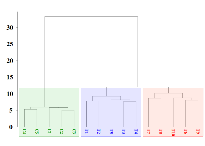
The statistical significance of the difference between two bisulfite sequence from control and treatment groups at each CG site can be evaluated with Fisher’s exact test. This is a statistical test used to determine if there are nonrandom associations between two categorical variables.

Let there exist two such (categorical) variables $X$ and $Y$, where $X$ stands for two groups of individuals: control and treatment, and $Y$ be a two states variable denoting the methylation status, carrying the number of times that a cytosine site is found methylated ($^{m}CG$) and non-methylated ($CG$), respectively.

This information can be summarized in a $2 \times 2$ table, a $2 \times 2$ matrix in which the entries $a_{ij}$ represent the number of observations in which $x=i$ and $y=j$. Calculate the row and column sums $R_i$ and $C_j$, respectively, and the total sum:

$N=\sum_iR_i=\sum_jC_j$

of the matrix:

  $Y = ^mCG$ $Y = CG$ $R_i$
Control $a_{11}$ $a_12$ $a_{11}+a_{12}$
Treatment $a_{21}$ $a_22$ $a_{21}+a_{22}$
$C_i$ $a_{11}+a_{21}$ $a_{12}+a_{22}$ $a_{11}+a_{12}+a_{21}+a_{22} = N$

Then the conditional probability of getting the actual matrix, given the particular row and column sums, is given by the formula:

$P_{cutoff}=\frac{R_1!R_2!}{N!\prod_{i,j}a_{ij}!}C_1!C_2!$

PCA and LDA with Methyl-IT

Principal Components and Linear Discriminant. Downstream Methylation Analyses with Methyl-IT

When methylation analysis is intended for diagnostic/prognostic purposes, for example, in clinical applications for patient diagnostics, to know whether the patient would be in healthy or disease stage we would like to have a good predictor tool in our side. It turns out that classical machine learning (ML) tools like hierarchical clustering, principal components and linear discriminant analysis can help us to reach such a goal. The current Methyl-IT downstream analysis is equipped with the mentioned ML tools.

1. Dataset

For the current example on methylation analysis with Methyl-IT we will use simulated data. Read-count matrices of methylated and unmethylated cytosine are generated with MethylIT.utils function simulateCounts. A basic example generating datasets is given in: Methylation analysis with Methyl-IT.

library(MethylIT) library(MethylIT.utils)
library(ggplot2)
library(ape)

alpha.ct <- 0.01
alpha.g1 <- 0.021
alpha.g2 <- 0.025

# The number of cytosine sites to generate
sites = 50000 
# Set a seed for pseudo-random number generation
set.seed(124)
control.nam <- c("C1", "C2", "C3", "C4", "C5")
treatment.nam1 <- c("T1", "T2", "T3", "T4", "T5")
treatment.nam2 <- c("T6", "T7", "T8", "T9", "T10")

# Reference group 
ref0 = simulateCounts(num.samples = 3, sites = sites, alpha = alpha.ct, beta = 0.5,
                      size = 50, theta = 4.5, sample.ids = c("R1", "R2", "R3"))
# Control group 
ctrl = simulateCounts(num.samples = 5, sites = sites, alpha = alpha.ct, beta = 0.5,
                      size = 50, theta = 4.5, sample.ids = control.nam)
# Treatment group II
treat = simulateCounts(num.samples = 5, sites = sites, alpha = alpha.g1, beta = 0.5,
                       size = 50, theta = 4.5, sample.ids = treatment.nam1)

# Treatment group II
treat2 = simulateCounts(num.samples = 5, sites = sites, alpha = alpha.g2, beta = 0.5,
                        size = 50, theta = 4.5, sample.ids = treatment.nam2)

A reference sample (virtual individual) is created using individual samples from the control population using function poolFromGRlist. The reference sample is further used to compute the information divergences of methylation levels, $TV_d$ and $H$, with function estimateDivergence [1]. This is a first fundamental step to remove the background noise (fluctuations) generated by the inherent stochasticity of the molecular processes in the cells.

# === Methylation level divergences ===
# Reference sample
ref = poolFromGRlist(ref0, stat = "mean", num.cores = 4L, verbose = FALSE)

divs <- estimateDivergence(ref = ref, indiv = c(ctrl, treat, treat2), Bayesian = TRUE, 
                           num.cores = 6L, percentile = 1, verbose = FALSE)

# To remove hd == 0 to estimate. The methylation signal only is given for  
divs = lapply(divs, function(div) div[ abs(div$hdiv) > 0 ], keep.attr = TRUE)
names(divs) <- names(divs)

To get some statistical description about the sample is useful. Here, empirical critical values for the probability distribution of $H$ and $TV_d$ is obtained using quantile function from the R package stats.

critical.val <- do.call(rbind, lapply(divs, function(x) {
  x <- x[x$hdiv > 0]
  hd.95 = quantile(x$hdiv, 0.95)
  tv.95 = quantile(abs(x$TV), 0.95)
  return(c(tv = tv.95, hd = hd.95))
}))
critical.val
##        tv.95%   hd.95%
## C1  0.2987088 21.92020
## C2  0.2916667 21.49660
## C3  0.2950820 21.71066
## C4  0.2985075 21.98416
## C5  0.3000000 22.04791
## T1  0.3376711 33.51223
## T2  0.3380282 33.00639
## T3  0.3387097 33.40514
## T4  0.3354077 31.95119
## T5  0.3402172 33.97772
## T6  0.4090909 38.05364
## T7  0.4210526 38.21258
## T8  0.4265781 38.78041
## T9  0.4084507 37.86892
## T10 0.4259411 38.60706

2. Modeling the methylation signal

Here, the methylation signal is expressed in terms of Hellinger divergence of methylation levels. Here, the signal distribution is modelled by a Weibull probability distribution model. Basically, the model could be a member of the generalized gamma distribution family. For example, it could be gamma distribution, Weibull, or log-normal. To describe the signal, we may prefer a model with a cross-validations: R.Cross.val > 0.95. Cross-validations for the nonlinear regressions are performed in each methylome as described in (Stevens 2009). The non-linear fit is performed through the function nonlinearFitDist.

The above statistical description of the dataset (evidently) suggests that there two main groups: control and treatments, while treatment group would split into two subgroups of samples. In the current case, to search for a good cutpoint, we do not need to use all the samples. The critical value $H_{\alpha=0.05}=33.51223$ suggests that any optimal cutpoint for the subset of samples T1 to T5 will be optimal for the samples T6 to T10 as well.

Below, we are letting the PCA+LDA model classifier to take the decision on whether a differentially methylated cytosine position is a treatment DMP. To do it, Methyl-IT function getPotentialDIMP is used to get methylation signal probabilities of the oberved $H$ values for all cytosine site (alpha = 1), in accordance with the 2-parameter Weibull distribution model. Next, this information will be used to identify DMPs using Methyl-IT function estimateCutPoint. Cytosine positions with $H$ values above the cutpoint are considered DMPs. Finally, a PCA + QDA model classifier will be fitted to classify DMPs into two classes: DMPs from control and those from treatment. Here, we fundamentally rely on a relatively strong $tv.cut \ge 0.34$ and on the signal probability distribution (nlms.wb) model.

dmps.wb <- getPotentialDIMP(LR = divs[1:10],
                             nlms = nlms.wb[1:10],  div.col = 9L, 
                             tv.cut = 0.34, tv.col = 7, alpha = 1, 
                             dist.name = "Weibull2P")
cut.wb = estimateCutPoint(LR = dmps.wb, simple = FALSE,
                            column = c(hdiv = TRUE, TV = TRUE, 
                                       wprob = TRUE, pos = TRUE),
                            classifier1 = "pca.lda", 
                             classifier2 = "pca.qda", tv.cut = 0.34,
                            control.names = control.nam, 
                            treatment.names = treatment.nam1,
                            post.cut = 0.5, cut.values = seq(15, 38, 1),
                            clas.perf = TRUE, prop = 0.6,
                            center = FALSE, scale = FALSE,
                            n.pc = 4, div.col = 9L, stat = 0)
cut.wb
## Cutpoint estimation with 'pca.lda' classifier 
## Cutpoint search performed using model posterior probabilities 
## 
## Posterior probability used to get the cutpoint = 0.5 
## Cytosine sites with treatment PostProbCut >= 0.5 have a 
## divergence value >= 3.121796 
## 
## Optimized statistic: Accuracy = 1 
## Cutpoint = 37.003 
## 
## Model classifier 'pca.qda' 
## 
## The accessible objects in the output list are: 
##                    Length Class           Mode     
## cutpoint           1      -none-          numeric  
## testSetPerformance 6      confusionMatrix list     
## testSetModel.FDR   1      -none-          numeric  
## model              2      pcaQDA          list     
## modelConfMatrix    6      confusionMatrix list     
## initModel          1      -none-          character
## postProbCut        1      -none-          numeric  
## postCut            1      -none-          numeric  
## classifier         1      -none-          character
## statistic          1      -none-          character
## optStatVal         1      -none-          numeric

The cutpoint is higher from what is expected from the higher treatment empirical critical value and DMPs are found for $H$ values: $H^{TT_{Emp}}_{\alpha=0.05}=33.98<37≤H$. The model performance in the whole dataset is:

# Model performance in in the whole dataset
cut.wb$modelConfMatrix
## Confusion Matrix and Statistics
## 
##           Reference
## Prediction   CT   TT
##         CT 4897    0
##         TT    2 9685
##                                      
##                Accuracy : 0.9999     
##                  95% CI : (0.9995, 1)
##     No Information Rate : 0.6641     
##     P-Value [Acc > NIR] : <2e-16     
##                                      
##                   Kappa : 0.9997     
##  Mcnemar's Test P-Value : 0.4795     
##                                      
##             Sensitivity : 1.0000     
##             Specificity : 0.9996     
##          Pos Pred Value : 0.9998     
##          Neg Pred Value : 1.0000     
##              Prevalence : 0.6641     
##          Detection Rate : 0.6641     
##    Detection Prevalence : 0.6642     
##       Balanced Accuracy : 0.9998     
##                                      
##        'Positive' Class : TT         
## 
# The False discovery rate
cut.wb$testSetModel.FDR
## [1] 0

3. Represeting individual samples as vectors from the N-dimensional space

The above cutpoint can be used to identify DMPs from control and treatment. The PCA+QDA model classifier can be used any time to discriminate control DMPs from those treatment. DMPs are retrieved using selectDIMP function:

dmps.wb <- selectDIMP(LR = divs, div.col = 9L, cutpoint = 37, tv.cut = 0.34, tv.col = 7)

Next, to represent individual samples as vectors from the N-dimensional space, we can use getGRegionsStat function from MethylIT.utils R package. Here, the simulated “chromosome” is split into regions of 450bp non-overlapping windows. and the density of Hellinger divergences values is taken for each windows.

ns <- names(dmps.wb)
DMRs <- getGRegionsStat(GR = dmps.wb, win.size = 450, step.size = 450, stat = "mean", column = 9L)
names(DMRs) <- ns

4. Hierarchical Clustering

Hierarchical clustering (HC) is an unsupervised machine learning approach. HC can provide an initial estimation of the number of possible groups and information on their members. However, the effectivity of HC will depend on the experimental dataset, the metric used, and the glomeration algorithm applied. For an unknown reason (and based on the personal experience of the author working in numerical taxonomy), Ward’s agglomeration algorithm performs much better on biological experimental datasets than the rest of the available algorithms like UPGMA, UPGMC, etc.
dmgm <- uniqueGRanges(DMRs, verbose = FALSE)
dmgm <- t(as.matrix(mcols(dmgm)))
rownames(dmgm) <- ns
sampleNames <- ns

hc = hclust(dist(data.frame( dmgm ))^2, method = 'ward.D')
hc.rsq = hc
hc.rsq$height <- sqrt( hc$height )4.

4.1. Dendrogram

colors = sampleNames 
colors[grep("C", colors)] <- "green4"
colors[grep("T[6-9]{1}", colors)] <- "red"
colors[grep("T10", colors)] <- "red"
colors[grep("T[1-5]", colors)] <- "blue"

# rgb(red, green, blue, alpha, names = NULL, maxColorValue = 1)
clusters.color = c(rgb(0, 0.7, 0, 0.1), rgb(0, 0, 1, 0.1), rgb(1, 0.2, 0, 0.1))

par(font.lab=2,font=3,font.axis=2, mar=c(0,3,2,0), family="serif" , lwd = 0.4)
plot(as.phylo(hc.rsq), tip.color = colors, label.offset = 0.5, font = 2, cex = 0.9,
     edge.width  = 0.4, direction = "downwards", no.margin = FALSE,
     align.tip.label = TRUE, adj = 0)
axisPhylo( 2, las = 1, lwd = 0.4, cex.axis = 1.4, hadj = 0.8, tck = -0.01 )
hclust_rect(hc.rsq, k = 3L, border = c("green4", "blue", "red"), 
            color = clusters.color, cuts = c(0.56, 15, 0.41, 300))

Here, we have use function as.phylo from the R package ape for better dendrogram visualization and function hclust_rect from MethylIT.utils R package to draw rectangles with background colors around the branches of a dendrogram highlighting the corresponding clusters.

5. PCA + LDA

MethylIT function pcaLDA will be used to perform the PCA and PCA + LDA analyses. The function returns a list of two objects: 1) ‘lda’: an object of class ‘lda’ from package ‘MASS’. 2) ‘pca’: an object of class ‘prcomp’ from package ‘stats’. For information on how to use these objects see ?lda and ?prcomp.

Unlike hierarchical clustering (HC), LDA is a supervised machine learning approach. So, we must provide a prior classification of the individuals, which can be derived, for example, from the HC, or from a previous exploratory analysis with PCA.

# A prior classification derived from HC
grps <- cutree(hc, k = 3)
grps[grep(1, grps)] <- "CT"
grps[grep(2, grps)] <- "T1"
grps[grep(3, grps)] <- "T2"
grps <- factor(grps)

ld <- pcaLDA(data = data.frame(dmgm), grouping = grps, n.pc = 3, max.pc = 3,
             scale = FALSE, center = FALSE, tol = 1e-6)
summary(ld$pca)
## Importance of first k=3 (out of 15) components:
## PC1 PC2 PC3
## Standard deviation 41.5183 4.02302 3.73302
## Proportion of Variance 0.9367 0.00879 0.00757
## Cumulative Proportion 0.9367 0.94546 0.95303

We may retain enough components so that the cumulative percent of variance accounted for at least 70 to 80% [2]. By setting $scale=TRUE$ and $center=TRUE$, we could have different results and would improve or not our results. In particular, these settings are essentials if the N-dimensional space is integrated by variables from different measurement scales/units, for example, Kg and g, or Kg and Km.

5.1. PCA

The individual coordinates in the principal components (PCs) are returned by function pcaLDA. In the current case, based on the cumulative proportion of variance, the two firsts PCs carried about the 94% of the total sample variance and could split the sample into meaningful groups.

pca.coord <- ld$pca$x
pca.coord
##           PC1         PC2        PC3
## C1 -21.74024 0.9897934 -1.1708548 ## C2 -20.39219 -0.1583025 0.3167283 ## C3 -21.19112 0.5833411 -1.1067609 ## C4 -21.45676 -1.4534412 0.3025241 ## C5 -21.28939 0.4152275 1.0021932 ## T1 -42.81810 1.1155640 8.9577860 ## T2 -43.57967 1.1712155 2.5135643 ## T3 -42.29490 2.5326690 -0.3136530 ## T4 -40.51779 0.2819725 -1.1850555 ## T5 -44.07040 -2.6172732 -4.2384395 ## T6 -50.03354 7.5276969 -3.7333568 ## T7 -50.08428 -10.1115700 3.4624095 ## T8 -51.07915 -5.4812595 -6.7778593 ## T9 -50.27508 2.3463125 3.5371351 ## T10 -51.26195 3.5405915 -0.9489265

5.2. Graphic PC1 vs PC2

Next, the graphic for individual coordinates in the two firsts PCs can be easely visualized now:

dt <- data.frame(pca.coord[, 1:2], subgrp = grps)

p0 <- theme(
  axis.text.x  = element_text( face = "bold", size = 18, color="black",
                               # hjust = 0.5, vjust = 0.5, 
                               family = "serif", angle = 0,
                               margin = margin(1,0,1,0, unit = "pt" )),
  axis.text.y  = element_text( face = "bold", size = 18, color="black", 
                               family = "serif",
                               margin = margin( 0,0.1,0,0, unit = "mm" )),
  axis.title.x = element_text(face = "bold", family = "serif", size = 18,
                              color="black", vjust = 0 ),
  axis.title.y = element_text(face = "bold", family = "serif", size = 18,
                              color="black", 
                              margin = margin( 0,2,0,0, unit = "mm" ) ),
  legend.title=element_blank(),
  legend.text = element_text(size = 20, face = "bold", family = "serif"),
  legend.position = c(0.899, 0.12),
  
  panel.border = element_rect(fill=NA, colour = "black",size=0.07),
  panel.grid.minor = element_line(color= "white",size = 0.2),
  axis.ticks = element_line(size = 0.1), axis.ticks.length = unit(0.5, "mm"),
  plot.margin = unit(c(1,1,0,0), "lines")) 

ggplot(dt, aes(x = PC1, y = PC2, colour = grps)) + 
  geom_vline(xintercept = 0, color = "white", size = 1) +
  geom_hline(yintercept = 0, color = "white", size = 1) +
  geom_point(size = 6) +
  scale_color_manual(values = c("green4","blue","brown1")) + 
  stat_ellipse(aes(x = PC1, y = PC2, fill = subgrp), data = dt, type = "norm",
               geom = "polygon", level = 0.5, alpha=0.2, show.legend = FALSE) +
  scale_fill_manual(values = c("green4","blue","brown1")) + p0

5.3. Graphic LD1 vs LD2

In the current case, better resolution is obtained with the linear discriminant functions, which is based on the three firsts PCs. Notice that the number principal components used the LDA step must be lower than the number of individuals ($N$) divided by 3: $N/3$.

ind.coord <- predict(ld, newdata = data.frame(dmgm), type = "scores")
dt <- data.frame(ind.coord, subgrp = grps)

p0 <- theme(
  axis.text.x  = element_text( face = "bold", size = 18, color="black",
                               # hjust = 0.5, vjust = 0.5, 
                               family = "serif", angle = 0,
                               margin = margin(1,0,1,0, unit = "pt" )),
  axis.text.y  = element_text( face = "bold", size = 18, color="black", 
                               family = "serif",
                               margin = margin( 0,0.1,0,0, unit = "mm" )),
  axis.title.x = element_text(face = "bold", family = "serif", size = 18,
                              color="black", vjust = 0 ),
  axis.title.y = element_text(face = "bold", family = "serif", size = 18,
                              color="black", 
                              margin = margin( 0,2,0,0, unit = "mm" ) ),
  legend.title=element_blank(),
  legend.text = element_text(size = 20, face = "bold", family = "serif"),
  legend.position = c(0.08, 0.12),
  
  panel.border = element_rect(fill=NA, colour = "black",size=0.07),
  panel.grid.minor = element_line(color= "white",size = 0.2),
  axis.ticks = element_line(size = 0.1), axis.ticks.length = unit(0.5, "mm"),
  plot.margin = unit(c(1,1,0,0), "lines")) 

ggplot(dt, aes(x = LD1, y = LD2, colour = grps)) + 
  geom_vline(xintercept = 0, color = "white", size = 1) +
  geom_hline(yintercept = 0, color = "white", size = 1) +
  geom_point(size = 6) +
  scale_color_manual(values = c("green4","blue","brown1")) + 
  stat_ellipse(aes(x = LD1, y = LD2, fill = subgrp), data = dt, type = "norm",
               geom = "polygon", level = 0.5, alpha=0.2, show.legend = FALSE) +
  scale_fill_manual(values = c("green4","blue","brown1")) + p0

References

  1. Liese, Friedrich, and Igor Vajda. 2006. “On divergences and informations in statistics and information theory.” IEEE Transactions on Information Theory 52 (10): 4394–4412. doi:10.1109/TIT.2006.881731.
  2. Stevens, James P. 2009. Applied Multivariate Statistics for the Social Sciences. Fifth Edit. Routledge Academic.

Methylation analysis with Methyl-IT. Part 2

 Methylation analysis with Methyl-IT is illustrated on simulated datasets of methylated and unmethylated read counts with relatively high average of  methylation levels: 0.15 and 0.286 for control and treatment groups, respectively. In this part, potential differentially methylated positions are estimated following different approaches.

1. Background

Only a signal detection approach can detect with high probability real DMPs. Any statistical test (like e.g. Fisher’s exact test) not based on signal detection requires for further analysis to distinguish DMPs that naturally can occur in the control group from those DMPs induced by a treatment. The analysis here is a continuation of Part 1.

2. Potential DMPs from the methylation signal using empirical distribution

As suggested from the empirical density graphics (above), the critical values $H_{\alpha=0.05}$ and $TV_{d_{\alpha=0.05}}$ can be used as cutpoints to select potential DMPs. After setting $dist.name = “ECDF”$ and $tv.cut = 0.926$ in Methyl-IT function getPotentialDIMP, potential DMPs are estimated using the empirical cummulative distribution function (ECDF) and the critical value $TV_{d_{\alpha=0.05}}=0.926$.

DMP.ecdf <- getPotentialDIMP(LR = divs, div.col = 9L, tv.cut = 0.926, tv.col = 7,
                            alpha = 0.05, dist.name = "ECDF")

3. Potential DMPs detected with Fisher’s exact test

In Methyl-IT Fisher’s exact test (FT) is implemented in function FisherTest. In the current case, a pairwise group application of FT to each cytosine site is performed. The differences between the group means of read counts of methylated and unmethylated cytosines at each site are used for testing (pooling.stat=”mean”). Notice that only cytosine sites with critical values $TV_d$> 0.926 are tested (tv.cut = 0.926).

ft = FisherTest(LR = divs, tv.cut = 0.926,
                     pAdjustMethod = "BH",  pooling.stat = "mean", 
                     pvalCutOff = 0.05, num.cores = 4L,
                     verbose = FALSE, saveAll = FALSE) 

ft.tv <- getPotentialDIMP(LR = ft, div.col = 9L, dist.name = "None",
                          tv.cut = 0.926, tv.col = 7, alpha = 0.05)

There is not a one-to-one mapping between $TV$ and $HD$. However, at each cytosine site $i$, these information divergences hold the inequality:

$TV(p^{tt}_i,p^{ct}_i)\leq \sqrt{2}H_d(p^{tt}_i,p^{ct}_i)$  [1].

where $H_d(p^{tt}_i,p^{ct}_i) = \sqrt{\frac{H(p^{tt}_i,p^{ct}_i)}w}$ is the Hellinger distance and $H(p^{tt}_i,p^{ct}_i)$ is given by Eq. 1 in part 1.
So, potential DMPs detected with FT can be constrained with the critical value $H^{TT}_{\alpha=0.05}\geq114.5$

4. Potential DMPs detected with Weibull 2-parameters model

Potential DMPs can be estimated using the critical values derived from the fitted Weibull 2-parameters models, which are obtained after the non-linear fit of the theoretical model on the genome-wide $HD$ values for each individual sample using Methyl-IT function nonlinearFitDist [2]. As before, only cytosine sites with critical values $TV>0.926$ are considered DMPs. Notice that, it is always possible to use any other values of $HD$ and $TV$ as critical values, but whatever could be the value it will affect the final accuracy of the classification performance of DMPs into two groups, DMPs from control and DNPs from treatment (see below). So, it is important to do an good choices of the critical values.

nlms.wb <- nonlinearFitDist(divs, column = 9L, verbose = FALSE, num.cores = 6L)
# Potential DMPs from 'Weibull2P' model
DMPs.wb <- getPotentialDIMP(LR = divs, nlms = nlms.wb, div.col = 9L, 
                            tv.cut = 0.926, tv.col = 7, alpha = 0.05, 
                            dist.name = "Weibull2P")
nlms.wb$T1 
##         Estimate   Std. Error  t value Pr(>|t|))      Adj.R.Square
## shape  0.5413711 0.0003964435 1365.570         0 0.991666592250838
## scale 19.4097502 0.0155797315 1245.833         0                  
##                     rho       R.Cross.val              DEV
## shape 0.991666258901194 0.996595712743823 34.7217494754823
## scale                                                     
##                     AIC               BIC     COV.shape     COV.scale
## shape -221720.747067975 -221694.287733122  1.571674e-07 -1.165129e-06
## scale                                     -1.165129e-06  2.427280e-04
##       COV.mu     n
## shape     NA 50000
## scale     NA 50000

5. Potential DMPs detected with Gamma 2-parameters model

As in the case of Weibull 2-parameters model, potential DMPs can be estimated using the critical values derived from the fitted Gamma 2-parameters models and only cytosine sites with critical values $TV_d > 0.926$ are considered DMPs.

nlms.g2p <- nonlinearFitDist(divs, column = 9L, verbose = FALSE, num.cores = 6L,
                            dist.name = "Gamma2P")
# Potential DMPs from 'Gamma2P' model
DMPs.g2p <- getPotentialDIMP(LR = divs, nlms = nlms.g2p,  div.col = 9L, 
                             tv.cut = 0.926, tv.col = 7, alpha = 0.05, 
                             dist.name = "Gamma2P")
nlms.g2p$T1
##         Estimate   Std. Error  t value Pr(>|t|))      Adj.R.Square
## shape  0.3866249 0.0001480347 2611.717         0 0.999998194156282
## scale 76.1580083 0.0642929555 1184.547         0                  
##                     rho       R.Cross.val                 DEV
## shape 0.999998194084045 0.998331895911125 0.00752417919133131
## scale                                                        
##                    AIC               BIC     COV.alpha     COV.scale
## shape -265404.29138371 -265369.012270572  2.191429e-08 -8.581717e-06
## scale                                    -8.581717e-06  4.133584e-03
##       COV.mu    df
## shape     NA 49998
## scale     NA 49998

Summary table:

data.frame(ft = unlist(lapply(ft, length)), ft.hd = unlist(lapply(ft.hd, length)),
ecdf = unlist(lapply(DMPs.hd, length)), Weibull = unlist(lapply(DMPs.wb, length)),
Gamma = unlist(lapply(DMPs.g2p, length)))
##      ft ft.hd ecdf Weibull Gamma
## C1 1253   773   63     756   935
## C2 1221   776   62     755   925
## C3 1280   786   64     768   947
## T1 2504  1554  126     924  1346
## T2 2464  1532  124     942  1379
## T3 2408  1477  121     979  1354

The graphics for the empirical (in black) and Gamma (in blue) densities distributions of Hellinger divergence of methylation levels for sample T1 are shown below. The 2-parameter gamma model is build by using the parameters estimated in the non-linear fit of $H$ values from sample T1. The critical values estimated from the 2-parameter gamma distribution $H^{\Gamma}_{\alpha=0.05}=124$ is more ‘conservative’ than the critical value based on the empirical distribution $H^{Emp}_{\alpha=0.05}=114.5$. That is, in accordance with the empirical distribution, for a methylation change to be considered a signal its $H$ value must be $H\geq114.5$, while according with the 2-parameter gamma model any cytosine carrying a signal must hold $H\geq124$.

suppressMessages(library(ggplot2))

# Some information for graphic
dt <- data[data$sample == "T1", ]
coef <- nlms.g2p$T1$Estimate # Coefficients from the non-linear fit
dgamma2p <- function(x) dgamma(x, shape = coef[1], scale = coef[2])
qgamma2p <- function(x) qgamma(x, shape = coef[1], scale = coef[2])

# 95% quantiles 
q95 <- qgamma2p(0.95) # Gamma model based quantile
emp.q95 = quantile(divs$T1$hdiv, 0.95) # Empirical quantile

# Density plot with ggplot
ggplot(dt, aes(x = HD)) + 
  geom_density(alpha = 0.05, bw = 0.2, position = "identity", na.rm = TRUE,
               size = 0.4) + xlim(c(0, 150)) +
  stat_function(fun = dgamma2p, colour = "blue") +
  xlab(expression(bolditalic("Hellinger divergence (HD)"))) + 
  ylab(expression(bolditalic("Density"))) +
  ggtitle("Empirical and Gamma densities distributions of Hellinger divergence (T1)") +
  geom_vline(xintercept = emp.q95, color = "black", linetype = "dashed", size = 0.4) +
  annotate(geom = "text", x = emp.q95 - 20, y = 0.16, size = 5,
           label = 'bolditalic(HD[alpha == 0.05]^Emp==114.5)',
           family = "serif", color = "black", parse = TRUE) +
  geom_vline(xintercept = q95, color = "blue", linetype = "dashed", size = 0.4) +
  annotate(geom = "text", x = q95 + 9, y = 0.14, size = 5,
           label = 'bolditalic(HD[alpha == 0.05]^Gamma==124)',
           family = "serif", color = "blue", parse = TRUE) +
  theme(
    axis.text.x  = element_text( face = "bold", size = 12, color="black",
                                 margin = margin(1,0,1,0, unit = "pt" )),
    axis.text.y  = element_text( face = "bold", size = 12, color="black", 
                                 margin = margin( 0,0.1,0,0, unit = "mm")),
    axis.title.x = element_text(face = "bold", size = 13,
                                color="black", vjust = 0 ),
    axis.title.y = element_text(face = "bold", size = 13,
                                color="black", vjust = 0 ),
    legend.title = element_blank(),
    legend.margin = margin(c(0.3, 0.3, 0.3, 0.3), unit = 'mm'),
    legend.box.spacing = unit(0.5, "lines"),
    legend.text = element_text(face = "bold", size = 12, family = "serif")
  1. Steerneman, Ton, K. Behnen, G. Neuhaus, Julius R. Blum, Pramod K. Pathak, Wassily Hoeffding, J. Wolfowitz, et al. 1983. “On the total variation and Hellinger distance between signed measures; an application to product measures.” Proceedings of the American Mathematical Society 88 (4). Springer-Verlag, Berlin-New York: 684–84. doi:10.1090/S0002-9939-1983-0702299-0.
  2. Sanchez, Robersy, and Sally A. Mackenzie. 2016. “Information Thermodynamics of Cytosine DNA Methylation.” Edited by Barbara Bardoni. PLOS ONE 11 (3). Public Library of Science: e0150427. doi:10.1371/journal.pone.0150427.

Methylation analysis with Methyl-IT. Part 1

 Methylation analysis with Methyl-IT is illustrated on simulated datasets of methylated and unmethylated read counts with relatively high average of  methylation levels: 0.15 and 0.286 for control and treatment groups, respectively. The main Methyl-IT downstream analysis is presented alongside the application of Fisher’s exact test. The importance of a signal detection step is shown.

Methyl-IT R package offers a methylome analysis approach based on information thermodynamics (IT) and signal detection. Methyl-IT approach confront detection of differentially methylated cytosine as a signal detection problem. This approach was designed to discriminate methylation regulatory signal from background noise induced by molecular stochastic fluctuations. Methyl-IT R package is not limited to the IT approach but also includes Fisher’s exact test (FT), Root-mean-square statistic (RMST) or Hellinger divergence (HDT) tests. Herein, we will show that a signal detection step is also required for FT, RMST, and HDT as well.

For the current example on methylation analysis with Methyl-IT we will use simulated data. Read count matrices of methylated and unmethylated cytosine are generated with Methyl-IT function simulateCounts. Function simulateCounts randomly generates prior methylation levels using Beta distribution function. The expected mean of methylation levels that we would like to have can be estimated using the auxiliary function:

bmean <- function(alpha, beta) alpha/(alpha + beta)
alpha.ct <- 0.09
alpha.tt <- 0.2
c(control.group = bmean(alpha.ct, 0.5), treatment.group = bmean(alpha.tt, 0.5), 
  mean.diff = bmean(alpha.tt, 0.5) - bmean(alpha.ct, 0.5)) 
##   control.group treatment.group       mean.diff 
##       0.1525424       0.2857143       0.1331719

This simple function uses the α and β (shape2) parameters from the Beta distribution function to compute the expected value of methylation levels. In the current case, we expect to have a difference of methylation levels about 0.133 between the control and the treatment.

Methyl-IT function simulateCounts will be used to generate the datasets, which will include three group of samples: reference, control, and treatment.

suppressMessages(library(MethylIT))

# The number of cytosine sites to generate
sites = 50000 
# Set a seed for pseudo-random number generation
set.seed(124)
control.nam <- c("C1", "C2", "C3")
treatment.nam <- c("T1", "T2", "T3")

# Reference group 
ref0 = simulateCounts(num.samples = 4, sites = sites, alpha = alpha.ct, beta = 0.5,
                      size = 50, theta = 4.5, sample.ids = c("R1", "R2", "R3"))
# Control group
ctrl = simulateCounts(num.samples = 3, sites = sites, alpha = alpha.ct, beta = 0.5,
                      size = 50, theta = 4.5, sample.ids = control.nam)
# Treatment group
treat = simulateCounts(num.samples = 3, sites = sites, alpha = alpha.tt, beta = 0.5,
                       size = 50, theta = 4.5, sample.ids = treatment.nam)

Notice that reference and control groups of samples are not identical but belong to the same population.

The estimation of the divergences of methylation levels is required to proceed with the application of signal detection basic approach. The information divergence is estimated here using the function estimateDivergence. For each cytosine site, methylation levels are estimated according to the formulas: $p_i={n_i}^{mC_j}/({n_i}^{mC_j}+{n_i}^{C_j})$, where ${n_i}^{mC_j}$ and ${n_i}^{C_j}$ are the number of methylated and unmethylated cytosines at site $i$.

If a Bayesian correction of counts is selected in function estimateDivergence, then methylated read counts are modeled by a beta-binomial distribution in a Bayesian framework, which accounts for the biological and sampling variations [1,2,3]. In our case we adopted the Bayesian approach suggested in reference [4] (Chapter 3).

Two types of information divergences are estimated: TV, total variation (TV, absolute value of methylation levels) and Hellinger divergence (H). TV is computed according to the formula: $TV=|p_{tt}-p_{ct}|$ and H:

$H(\hat p_{ij},\hat p_{ir}) = w_i[(\sqrt{\hat p_{ij}} – \sqrt{\hat p_{ir}})^2+(\sqrt{1-\hat p_{ij}} – \sqrt{1-\hat p_{ir}})^2]$  (1)

where $w_i = 2 \frac{m_{ij} m_{ir}}{m_{ij} + m_{ir}}$, $m_{ij} = {n_i}^{mC_j}+{n_i}^{uC_j}+1$, $m_{ir} = {n_i}^{mC_r}+{n_i}^{uC_r}+1$ and $j \in {\{c,t}\}$

The equation for Hellinger divergence is given in reference [5], but
any other information theoretical divergences could be used as well. Divergences are estimated for control and treatment groups in respect to a virtual sample, which is created applying function poolFromGRlist on the reference group.

.

# Reference sample
ref = poolFromGRlist(ref0, stat = "mean", num.cores = 4L, verbose = FALSE)

# Methylation level divergences
DIVs <- estimateDivergence(ref = ref, indiv = c(ctrl, treat), Bayesian = TRUE, 
                           num.cores = 6L, percentile = 1, verbose = FALSE)

The mean of methylation levels differences is:

unlist(lapply(DIVs, function(x) mean(mcols(x[, 7])[,1])))
##            C1            C2            C3            T1            T2 
## -0.0009820776 -0.0014922009 -0.0022257725  0.1358867135  0.1359160219 
##            T3 
##  0.1309217360

Likewise for any other signal in nature, the analysis of methylation signal requires for the knowledge of its probability distribution. In the current case, the signal is represented in terms of the Hellinger divergence of methylation levels (H).

divs = DIVs[order(names(DIVs))]

# To remove hd == 0 to estimate. The methylation signal only is given for  
divs = lapply(divs, function(div) div[ abs(div$hdiv) > 0 ])
names(divs) <- names(DIVs)

# Data frame with the Hellinger divergences from both groups of samples samples 
l = c(); for (k in 1:length(divs)) l = c(l, length(divs[[k]]))
data <- data.frame(H = c(abs(divs$C1$hdiv), abs(divs$C2$hdiv), abs(divs$C3$hdiv),
                           abs(divs$T1$hdiv), abs(divs$T2$hdiv), abs(divs$T3$hdiv)),
                   sample = c(rep("C1", l[1]), rep("C2", l[2]), rep("C3", l[3]),
                              rep("T1", l[4]), rep("T2", l[5]), rep("T3", l[6]))
)

Empirical critical values for the probability distribution of H and TV can be obtained using quantile function from the R package stats.

critical.val <- do.call(rbind, lapply(divs, function(x) {
  hd.95 = quantile(x$hdiv, 0.95)
  tv.95 = quantile(x$TV, 0.95)
  return(c(tv = tv.95, hd = hd.95))
}))

critical.val
##       tv.95%    hd.95%
## C1 0.7893927  81.47256
## C2 0.7870469  80.95873
## C3 0.7950869  81.27145
## T1 0.9261629 113.73798
## T2 0.9240506 114.45228
## T3 0.9212163 111.54258

3.1. Density estimation

The kernel density estimation yields the empirical density shown in the graphics:

suppressMessages(library(ggplot2))

# Some information for graphic
crit.val.ct <- max(critical.val[c("C1", "C2", "C3"), 2]) # 81.5
crit.val.tt <- min(critical.val[c("T1", "T2", "T3"), 2]) # 111.5426

# Density plot with ggplot
ggplot(data, aes(x = H, colour = sample, fill = sample)) + 
  geom_density(alpha = 0.05, bw = 0.2, position = "identity", na.rm = TRUE,
               size = 0.4) + xlim(c(0, 125)) +   
  xlab(expression(bolditalic("Hellinger divergence (H)"))) + 
  ylab(expression(bolditalic("Density"))) +
  ggtitle("Density distribution for control and treatment") +
  geom_vline(xintercept = crit.val.ct, color = "red", linetype = "dashed", size = 0.4) +
  annotate(geom = "text", x = crit.val.ct-2, y = 0.3, size = 5,
           label = 'bolditalic(H[alpha == 0.05]^CT==81.5)',
           family = "serif", color = "red", parse = TRUE) +
  geom_vline(xintercept = crit.val.tt, color = "blue", linetype = "dashed", size = 0.4) +
  annotate(geom = "text", x = crit.val.tt -2, y = 0.2, size = 5,
           label = 'bolditalic(H[alpha == 0.05]^TT==114.5)',
           family = "serif", color = "blue", parse = TRUE) +
  theme(
    axis.text.x  = element_text( face = "bold", size = 12, color="black",
                                 margin = margin(1,0,1,0, unit = "pt" )),
    axis.text.y  = element_text( face = "bold", size = 12, color="black", 
                                 margin = margin( 0,0.1,0,0, unit = "mm")),
    axis.title.x = element_text(face = "bold", size = 13,
                                color="black", vjust = 0 ),
    axis.title.y = element_text(face = "bold", size = 13,
                                color="black", vjust = 0 ),
    legend.title = element_blank(),
    legend.margin = margin(c(0.3, 0.3, 0.3, 0.3), unit = 'mm'),
    legend.box.spacing = unit(0.5, "lines"),
    legend.text = element_text(face = "bold", size = 12, family = "serif")
  )
The above graphic shows that with high probability the methylation signal induced by the treatment has H values $H^{TT}_{\alpha=0.05}\geq114.5$. According to the critical value estimated for the differences of methylation levels, the methylation signal holds $TV^{TT}_{\alpha=0.05}\geq0.926$. Notice that most of the methylation changes are not signal but noise (found to the left of the critical values). This situation is typical for all the natural and technologically generated signals. Assuming that the background methylation variation is consistent with a Poisson process and that methylation changes conform to the second law of thermodynamics, the Hellinger divergence of methylation levels follows a Weibull distribution probability or some member of the generalized gamma distribution family [6].
  1. Hebestreit, Katja, Martin Dugas, and Hans-Ulrich Klein. 2013. “Detection of significantly differentially methylated regions in targeted bisulfite sequencing data.” Bioinformatics (Oxford, England) 29 (13): 1647–53. doi:10.1093/bioinformatics/btt263.
  2. Hebestreit, Katja, Martin Dugas, and Hans-Ulrich Klein. 2013. “Detection of significantly differentially methylated regions in targeted bisulfite sequencing data.” Bioinformatics (Oxford, England) 29 (13): 1647–53. doi:10.1093/bioinformatics/btt263.
  3. Dolzhenko, Egor, and Andrew D Smith. 2014. “Using beta-binomial regression for high-precision differential methylation analysis in multifactor whole-genome bisulfite sequencing experiments.” BMC Bioinformatics 15 (1). BioMed Central: 215. doi:10.1186/1471-2105-15-215.
  4. Baldi, Pierre, and Soren Brunak. 2001. Bioinformatics: the machine learning approach. Second. Cambridge: MIT Press.
  5. Basu, A., A. Mandal, and L. Pardo. 2010. “Hypothesis testing for two discrete populations based on the Hellinger distance.” Statistics & Probability Letters 80 (3-4). Elsevier B.V.: 206–14. doi:10.1016/j.spl.2009.10.008.
  6. Sanchez R, Mackenzie SA. Information Thermodynamics of Cytosine DNA Methylation. PLoS One, 2016, 11:e0150427.