Fitting Mixture Distributions
1. Background
Mixture Distributions were introduced in a previous post. Basically, it is said that a distribution $f(x)$ is a mixture of k components distributions $f_1(x), …, f_k(x)$ if:
$f(x) = \sum_{i=1}^k \pi_i f_i(x)$
where $\pi_i$ are the so called mixing weights, $0 \le \pi_i \le 1$, and $\pi_1 + … + \pi_k = 1$. Here, new data points from distribution will be generated in the standard way: first to pick a distribution, with probabilities given by the mixing weights, and then to generate one observation according to that distribution. More information about mixture distribution can be read in Wikipedia.
Herein, we will show how to fit numerical data to a mixture of probability distributions model.
2. Generating random variables from a mixture of Gamma and Weibull distributions
To generate from a mixture distribution the R package usefr will be used.
library(usefr)set.seed(123) # set a seed for random generation
# ========= A mixture of three distributions =========phi = c(3/10, 7/10) # Mixture proportions# ---------------------------------------------------------# === Named vector of the corresponding distribution function parameters# must be providedargs <- list(gamma = c(shape = 2, scale = 0.1),
weibull = c(shape = 3, scale = 0.5))# ------------------------------------------------------------# ===== Sampling from the specified mixture distribution ====X <- rmixtdistr(n = 1e5, phi = phi , arg = args)
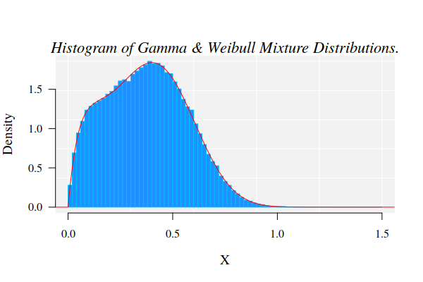
2.1. The histogram of the mixture distribution
The graphics for the simulated dataset and the corresponding theoretical mixture distribution
hist(X, 90, freq = FALSE, las = 1, family = "serif",
panel.first={points(0, 0, pch=16, cex=1e6, col="grey95")
grid(col="white", lty = 1)}, family = "serif", col = "cyan1",
border = "deepskyblue", xlim = c(0, 1.5))
x1 <- seq(-4, 1.5, by = 0.001)
lines(x1, dmixtdistr(x1, phi = phi, arg = args), col = "red")

The nonlinear fit of this dataset is NOT straightforward!
3. Nonlinear fit of the random generated dataset
The nonlinear fit of the random generated data set will be accomplished with the function fitMixDist.
FIT <- fitMixDist(X, args = list(gamma = c(shape = NULL, scale = NULL),weibull = c(shape = NULL, scale = NULL)),npoints = 200, usepoints = 1000)
fitting ...
|========================================================================================================| 100
summary(FIT$fit)#> Parameters:
#> Estimate Std. Error t value Pr(>|t|)
#> gamma.shape 1.828989 0.021444 85.29 <2e-16 ***
#> gamma.scale 6.058377 0.108738 55.72 <2e-16 ***
#> weibull.shape 3.449296 0.025578 134.85 <2e-16 ***
#> weibull.scale 0.507976 0.001461 347.66 <2e-16 ***
#> ---
#> Signif. codes: 0 ‘***’ 0.001 ‘**’ 0.01 ‘*’ 0.05 ‘.’ 0.1 ‘ ’ 1
#> Residual standard error: 0.02403 on 71 degrees of freedom
#> Number of iterations to termination: 27
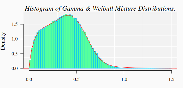
#> Reason for termination: Relative error in the sum of squares is at most `ftol'. 3.1. Graphics of the simulated dataset and the corresponding theoretical mixture distribution
hist(X, 90, freq = FALSE, las = 1, family = "serif",
panel.first={points(0, 0, pch=16, cex=1e6, col="grey95")
grid(col="white", lty = 1)}, family = "serif", col = "seagreen1",
border = "deepskyblue", xlim = c(0, 1.5), cex.lab = 1.2)
x1 <- seq(-4, 10, by = 0.001)
lines(x1, dmixtdistr(x1, phi = FIT$phi, arg = FIT$args), col = "red")
mtext("Histogram of Gamma & Weibull Mixture Distributions.", cex = 1.4, font = 3, family = "serif")
3.2. Bootstrap goodness-of-fit test
A bootstrap goodness-of-fit (GOF) test is performed with function mcgoftest.
The parameter values are taken from the previous fitted mixture distribution model. Notice the particular way to set up the list of parameters. The Null hypothesis is that the data set follows a mixture of Gamma and Weibull distributions with the estimated parameter values.
pars <- c(list(phi = FIT$phi), arg = list(FIT$args))
mcgoftest(varobj = X, distr = "mixtdistr", pars = pars, num.sampl = 999,
          sample.size = 99999, stat = "chisq", num.cores = 4, breaks = 200, seed = 123)
#> *** Monte Carlo GoF testing based on Pearson's Chi-squared statistic ( parametric approach ) ...
#> Chisq mc_p.value sample.size num.sampl
#> 815.1484 0.0010 99999.0000 999.0000
The GOF rejected the null hypothesis. In particular, the computation yielded several warnings about the fitting of Gamma distribution. Nevertheless, we can use the previous estimated parameter values to “guess” better starting values for the fitting algorithm:
FIT <- fitMixDist(X, args = list(gamma = c(shape = 1.8, scale = 6),
weibull = c(shape = 3, scale = 0.5)), npoints = 200, usepoints = 1000)
summary(FIT$fit)
#> fitting ...
#>  |======================================================================================================================| 100
#> *** Performing nonlinear regression model  crossvalidation...
#> Warning messages:
#> 1: In dgamma(c(0.005, 0.015, 0.025, 0.035, 0.045, 0.055, 0.065, 0.075,  :
#>  NaNs produced
#> 2: In dgamma(c(0.005, 0.015, 0.025, 0.035, 0.045, 0.055, 0.065, 0.075,  :
#>  NaNs produced
#> 3: In dgamma(c(0.005, 0.015, 0.025, 0.035, 0.045, 0.055, 0.065, 0.075,  :
#>  NaNs produced

#> Parameters:
#>               Estimate Std. Error t value Pr(>|t|)
#> gamma.shape   2.0050960  0.0265535   75.51   <2e-16 ***
#> gamma.scale   0.0953489  0.0017654   54.01   <2e-16 ***
#> weibull.shape 2.9221485  0.0127682  228.86   <2e-16 ***
#> weibull.scale 0.4957061  0.0007669  646.41   <2e-16 ***
#> ---
#> Signif. codes:  0 ‘***’ 0.001 ‘**’ 0.01 ‘*’ 0.05 ‘.’ 0.1 ‘ ’ 1

#> Residual standard error: 0.02681 on 145 degrees of freedom
#> Number of iterations to termination: 17
#> Reason for termination: Relative error in the sum of squares is at most `ftol'.
The GOF test is now repeated with new estimated parameter values:
pars <- c(list(phi = FIT$phi), arg = list(FIT$args))
mcgoftest(varobj = X, distr = "mixtdistr", pars = pars, num.sampl = 999,
          sample.size = 99999, stat = "chisq", num.cores = 4, breaks = 200, seed = 123)
*** Monte Carlo GoF testing based on Pearson's Chi-squared statistic ( parametric approach ) ...
Chisq mc_p.value sample.size num.sampl
111.3769 0.9150 99999.0000 999.0000 That is, for the last estimated parameters, there is not enough statistical reasons to reject the null hypothesis. Although the corresponding histogram looks pretty similar to the previous ones, the numbers indicate that there small fitting differences that our eyes cannot detect in the graphics.