Fisher's exact test failure can lead to biased results

Robersy Sanchez

Department of Biology. Pennsylvania State University, University Park, PA 16802

Email: rus547@psu.edu

Fisher’s exact test is a statistical significance test used in the analysis of contingency tables. Although this test is routinely used even though, it has been full of with controversy for over 80 years. Herein, the case of its application analyzed is scrutinized with specific examples.

Overwiew

The statistical significance of the difference between two bisulfite sequence from control and treatment groups at each CG site can be evaluated with Fisher’s exact test. This is a statistical test used to determine if there are nonrandom associations between two categorical variables.

Let there exist two such (categorical) variables $X$ and $Y$, where $X$ stands for two groups of individuals: control and treatment, and $Y$ be a two states variable denoting the methylation status, carrying the number of times that a cytosine site is found methylated ($^{m}CG$) and non-methylated ($CG$), respectively.

This information can be summarized in a $2 \times 2$ table, a $2 \times 2$ matrix in which the entries $a_{ij}$ represent the number of observations in which $x=i$ and $y=j$. Calculate the row and column sums $R_i$ and $C_j$, respectively, and the total sum:

$N=\sum_iR_i=\sum_jC_j$

of the matrix:

  $Y = ^mCG$ $Y = CG$ $R_i$
Control $a_{11}$ $a_12$ $a_{11}+a_{12}$
Treatment $a_{21}$ $a_22$ $a_{21}+a_{22}$
$C_i$ $a_{11}+a_{21}$ $a_{12}+a_{22}$ $a_{11}+a_{12}+a_{21}+a_{22} = N$

Then the conditional probability of getting the actual matrix, given the particular row and column sums, is given by the formula:

$P_{cutoff}=\frac{R_1!R_2!}{N!\prod_{i,j}a_{ij}!}C_1!C_2!$
Non-linear Fit of Mixture Distributions

Fitting Mixture Distributions

1. Background

Mixture Distributions were introduced in a previous postBasically, it is said that a distribution $f(x)$ is a mixture of k components distributions $f_1(x), …, f_k(x)$ if:

$f(x) = \sum_{i=1}^k \pi_i f_i(x)$

where $\pi_i$ are the so called mixing weights, $0 \le \pi_i \le 1$, and $\pi_1 + … + \pi_k = 1$. Here, new data points from distribution will be generated in the standard way: first to pick a distribution, with probabilities given by the mixing weights, and then to generate one observation according to that distribution. More information about mixture distribution can be read in Wikipedia.

Herein, we will show how to fit numerical data to a mixture of probability distributions model.

2. Generating random variables from a mixture of Gamma and Weibull distributions

To generate from a mixture distribution the R package usefr will be used.

library(usefr) 
set.seed(123) # set a seed for random generation
# ========= A mixture of three distributions =========
phi = c(3/10, 7/10) # Mixture proportions
# ---------------------------------------------------------
# === Named vector of the corresponding distribution function parameters
# must be provided
args <- list(gamma = c(shape = 2, scale = 0.1),
weibull = c(shape = 3, scale = 0.5))

# ------------------------------------------------------------
# ===== Sampling from the specified mixture distribution ====
X <- rmixtdistr(n = 1e5, phi = phi , arg = args)

2.1. The histogram of the mixture distribution

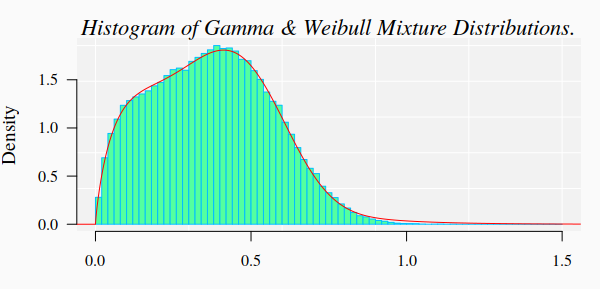
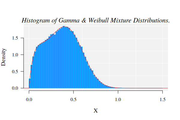
The graphics for the simulated dataset and the corresponding theoretical mixture distribution

hist(X, 90, freq = FALSE, las = 1, family = "serif", 
panel.first={points(0, 0, pch=16, cex=1e6, col="grey95")
grid(col="white", lty = 1)}, family = "serif", col = "cyan1",
border = "deepskyblue", xlim = c(0, 1.5))
x1 <- seq(-4, 1.5, by = 0.001)
lines(x1, dmixtdistr(x1, phi = phi, arg = args), col = "red")

The nonlinear fit of this dataset is NOT straightforward!

3. Nonlinear fit of the random generated dataset

The nonlinear fit of the random generated data set will be accomplished with the function fitMixDist.

FIT <- fitMixDist(X, args = list(gamma = c(shape = NULL, scale = NULL),
weibull = c(shape = NULL, scale = NULL)),
npoints = 200, usepoints = 1000)
fitting ...
|========================================================================================================| 100%
*** Performing nonlinear regression model crossvalidation...
Warning messages:
1: In dgamma(c(0.005, 0.015, 0.025, 0.035, 0.045, 0.055, 0.065, 0.075, :
NaNs produced
2: In dgamma(c(0.005, 0.015, 0.025, 0.035, 0.045, 0.055, 0.065, 0.075, :
NaNs produced
3: In dgamma(c(0.005, 0.015, 0.025, 0.035, 0.045, 0.055, 0.065, 0.075, :
NaNs produced
summary(FIT$fit)
#> Parameters:
#>               Estimate Std. Error t value Pr(>|t|)    
#> gamma.shape   1.828989   0.021444   85.29   <2e-16 ***
#> gamma.scale   6.058377   0.108738   55.72   <2e-16 ***
#> weibull.shape 3.449296   0.025578  134.85   <2e-16 ***
#> weibull.scale 0.507976   0.001461  347.66   <2e-16 ***
#> ---
#> Signif. codes:  0 ‘***’ 0.001 ‘**’ 0.01 ‘*’ 0.05 ‘.’ 0.1 ‘ ’ 1

#> Residual standard error: 0.02403 on 71 degrees of freedom
#> Number of iterations to termination: 27 
#> Reason for termination: Relative error in the sum of squares is at most `ftol'. 

3.1. Graphics of the simulated dataset and the corresponding theoretical mixture distribution

hist(X, 90, freq = FALSE, las = 1, family = "serif", 
panel.first={points(0, 0, pch=16, cex=1e6, col="grey95")
grid(col="white", lty = 1)}, family = "serif", col = "seagreen1",
border = "deepskyblue", xlim = c(0, 1.5), cex.lab = 1.2)
x1 <- seq(-4, 10, by = 0.001)
lines(x1, dmixtdistr(x1, phi = FIT$phi, arg = FIT$args), col = "red")
mtext("Histogram of Gamma & Weibull Mixture Distributions.", cex = 1.4, font = 3, family = "serif")

3.2. Bootstrap goodness-of-fit test

A bootstrap goodness-of-fit (GOF) test is performed with function mcgoftest.

The parameter values are taken from the previous fitted mixture distribution model. Notice the particular way to set up the list of parameters. The Null hypothesis is that the data set follows a mixture of Gamma and Weibull distributions with the estimated parameter values. 

pars <- c(list(phi = FIT$phi), arg = list(FIT$args))
mcgoftest(varobj = X, distr = "mixtdistr", pars = pars, num.sampl = 999,
sample.size = 99999, stat = "chisq", num.cores = 4, breaks = 200, seed = 123)
#> *** Monte Carlo GoF testing based on Pearson's Chi-squared statistic ( parametric approach )  ...
#>      Chisq  mc_p.value sample.size   num.sampl 
#>   815.1484      0.0010​  99999.0000    999.0000

The GOF rejected the null hypothesis. In particular, the computation yielded several warnings about the fitting of Gamma distribution. Nevertheless, we can use the previous estimated parameter values to “guess” better starting values for the fitting algorithm:

FIT <- fitMixDist(X, args = list(gamma = c(shape = 1.8, scale = 6),
weibull = c(shape = 3, scale = 0.5)), npoints = 200, usepoints = 1000)
summary(FIT$fit)
#> fitting ...
#>  |======================================================================================================================| 100%
#> *** Performing nonlinear regression model  crossvalidation...
#> Warning messages:
#> 1: In dgamma(c(0.005, 0.015, 0.025, 0.035, 0.045, 0.055, 0.065, 0.075,  :
#>  NaNs produced
#> 2: In dgamma(c(0.005, 0.015, 0.025, 0.035, 0.045, 0.055, 0.065, 0.075,  :
#>  NaNs produced
#> 3: In dgamma(c(0.005, 0.015, 0.025, 0.035, 0.045, 0.055, 0.065, 0.075,  :
#>  NaNs produced
#> Parameters: #> Estimate Std. Error t value Pr(>|t|) #> gamma.shape 2.0050960 0.0265535 75.51 <2e-16 *** #> gamma.scale 0.0953489 0.0017654 54.01 <2e-16 *** #> weibull.shape 2.9221485 0.0127682 228.86 <2e-16 *** #> weibull.scale 0.4957061 0.0007669 646.41 <2e-16 *** #> --- #> Signif. codes: 0 ‘***’ 0.001 ‘**’ 0.01 ‘*’ 0.05 ‘.’ 0.1 ‘ ’ 1 #> Residual standard error: 0.02681 on 145 degrees of freedom #> Number of iterations to termination: 17 #> Reason for termination: Relative error in the sum of squares is at most `ftol'.

The GOF test is now repeated with new estimated parameter values:

pars <- c(list(phi = FIT$phi), arg = list(FIT$args))
mcgoftest(varobj = X, distr = "mixtdistr", pars = pars, num.sampl = 999,
sample.size = 99999, stat = "chisq", num.cores = 4, breaks = 200, seed = 123)
*** Monte Carlo GoF testing based on Pearson's Chi-squared statistic ( parametric approach )  ...
      Chisq  mc_p.value sample.size   num.sampl 
   111.3769      0.9150  99999.0000    999.0000 

That is, for the last estimated parameters, there is not enough statistical reasons to reject the null hypothesis. Although the corresponding histogram looks pretty similar to the previous ones, the numbers indicate that there small fitting differences that our eyes cannot detect in the graphics.

Sampling from a Mixture of Distributions

Sampling from a Mixture of Distributions

It is said that a distribution $f(x)$ is a mixture of k components distributions $f_1(x), …, f_k(x)$ if:

$f(x) = \sum_{i=1}^k \pi_i f_i(x)$

where $\pi_i$ are the so called mixing weights, $0 \le \pi_i \le 1$, and $\pi_1 + … + \pi_k = 1$. Here, new data points from distribution will be generated in the standard way: first to pick a distribution, with probabilities given by the mixing weights, and then to generate one observation according to that distribution. More information about mixture distribution can be read in Wikipedia.

1. Generating random variables from a mixture of normal distributions

To generate from a mixture distribution the R package usefr will be used.

library(usefr)
set.seed(123) # set a seed for random generation

# ========= A mixture of three distributions =========
phi = c(7/10, 3/10) # Mixture proportions
# ---------------------------------------------------------

# === Named vector of the corresponding distribution function parameters
# must be provided
args <- list(norm = c(mean = 1, sd = 1), norm = c(mean = 5, sd = 1))
# ------------------------------------------------------------

# ===== Sampling from the specified mixture distribution ====
x <- rmixtdistr(n = 1e5, pi = pi , arg = args)
# ------------------------------------------------------------


# === The graphics for the simulated dataset and the corresponding theoretical

# mixture distribution
par(bg = "gray98", mar = c(3, 4, 2, 1) )
hist(x, 90, freq = FALSE, las = 1, family = "serif", col = rgb(0, 0, 1, 0.2), border = "deepskyblue")
x1 <- seq(-4, 10, by = 0.001)
lines(x1, dmixtdistr(x1, phi = phi, arg = args), col = "red")

2. Mixture of Weibull and Gamma distributions

Mixture of normal distributions is what most frequently we see online and in paper. Let’s see the mixture of Weibull and Gamma distributions.

set.seed(123) # set a seed for random generation 
# ==== A mixture of three distributions =====
pi = c(7/10, 3/10) # Mixture proportions # --------------------------------------------------------- # === Named vector of the corresponding distribution function parameters
 # must be provided
args <- list(gamma = c(shape = 20, scale = 1/15), weibull = c(shape = 3, scale = 0.5))
# ---------------------------------------------------------
# === Sampling from the specified mixture distribution ====

 x <- rmixtdistr(n = 1e5, pi = pi , arg = args)
# ---------------------------------------------------------
# === The graphics for the simulated dataset and the corresponding theoretical

# mixture distribution
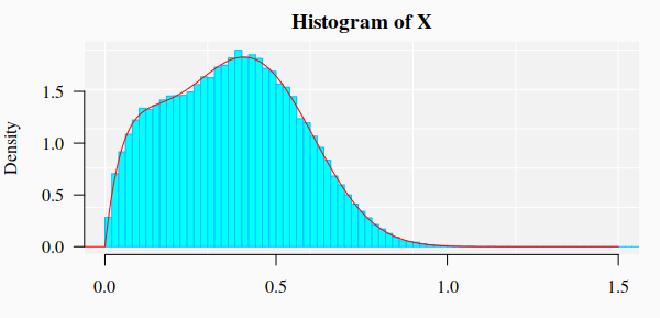
par(bg = "gray98", mar = c(3, 4, 2, 1) )
hist(x, 90, freq = FALSE, las = 1, family = "serif", col = "cyan1", border = "deepskyblue")
x1 <- seq(-4, 10, by = 0.001)
 lines(x1, dmixtdistr(x1, pi = pi, arg = args), col = "red")

3. Mixture of Gamma, Weibull, and Log-Normal distributions


set.seed(123) # set a seed for random generation
# =============== A mixture of three distributions ========================
pi = c(5/10, 3/10, 2/10) # Mixture proportions
# --------------------------------------------------------------------------
# ==== Named vector of the corresponding distribution function parameters
# must be provided
args <- list(gamma = c(shape = 20, scale = 1/10),
weibull = c(shape = 4, scale = 0.8),
lnorm = c(meanlog = 1.2, sdlog = 0.08))
# --------------------------------------------------------------------------
# ======= Sampling from the specified mixture distribution =======
x <- rmixtdistr(n = 1e5, pi = pi , arg = args)
# --------------------------------------------------------------------------
# The graphics for the simulated dataset and the corresponding theoretical
# mixture distribution
par(bg = "gray98", mar = c(3, 4, 2, 1) )
hist(x, 90, freq = FALSE, las = 1, family = "serif", col = "plum1", border = "violet")
x1 <- seq(-4, 10, by = 0.001)
lines(x1, dmixtdistr(x1, pi = pi, arg = args), col = "red")

Monte-Carlo Goodness of Fit Test

Goodness of fit with large Sample size

1. Background

The goodness of fit (GOF) tests frequently fail with real datasets when the sample size goes beyond 100. This issue is critical when working with experimental data where enviromental random noise cannot be prevented. Fortunately, permutation and Monte Carlo approaches for GOF could help to confront the issue. Herein, two examples with simulated data are presented.

2. Install and loading the R packages needed for the computation

To run a Monte Carlo (MC) approach for GOF we will install the R package usefr and its dependences from GitHub:

source("https://bioconductor.org/biocLite.R")
biocLite('BiocParallel')
install.packages(c("minpack.lm", "numDeriv", "devtools", "ggplot2", "gridExtra"), 
                 dependencies=TRUE)
devtools::install_git("https://github.com/genomaths/usefr.git")

Next, to load the packages that are needed for this example:

suppressMessages(library(ggplot2))
suppressMessages(library(gridExtra))
suppressMessages(library(usefr))

2. Example 1

Let us simulate random samples from a specified Normal and Weibull distributions. To make reproducible this example, we set a seed.

set.seed(1)
x1 = rnorm(10000, mean = 1.5, sd = 2)
x2 = rweibull(10000, shape = 0.5, scale = 1.2)
dt <- data.frame(x1 = x1, x2 = x2)

2.1 The histograms and density plots of the given Normal and Weibull distributions

p1 <- ggplot(data = dt, aes(x1)) + 
  geom_histogram(data = dt, aes(y=..density..), binwidth = 1, 
                 colour = "black", fill = "skyblue", na.rm=TRUE) +
  stat_function(fun = dnorm, n = 101, col = "red",
                args = list(mean = 1.5, sd = 2), size = 1) +
  theme_gray(base_family = "serif", base_size = 14) +
  annotate(geom = "text", x = 7, y = 0.16, size = 6,
           label = 'bolditalic(N(1.5,2))',
           family = "serif", color = "blue", parse = TRUE)  

p2 <- ggplot(data = dt, aes(x2)) + 
  geom_histogram(data = dt, aes(y=..density..), binwidth = 1, 
                 colour = "black", fill = "skyblue", na.rm=TRUE) + 
  xlim(0,20) + ylim(0,0.23) +
  stat_function(fun = dweibull, n = 101, col = "red",
                args = list(shape = 0.5, scale = 1.2), size = 1) +
  theme_gray(base_family = "serif", base_size = 14) +
  annotate(geom = "text", x = 10, y = 0.18, size = 6,
           label = 'bolditalic(W(0.5, 1.2))',
           family = "serif", color = "blue", parse = TRUE)
grid.arrange(p1, p2, nrow = 1)

The bell shape, typical of the normal distribution, is clear. Many people are not familiar with the Weibull distribution. The decay observed in the Weibull distribution presented in the figure is typically found for the for information divergences of DNA methylation levels, in humans and in plants [1].

3. The Monte Carlo GOF test

The test is performed with function mcgoftest from the R package usefr

mcgoftest(x1, cdf = pnorm, pars = c(1.5, 2), num.sampl = 500,
          sample.size = 1000, num.cores = 1)
## *** Monte Carlo GoF testing based on Kolmogorov-Smirnov statistic ...
## KS.stat.D mc_p.value KS.stat.p.value sample.size num.sampl
## 0.2534276 0.6007984 0.0000000 1000.0000000 500.0000000

Kolmogorov-Smirnov (KS) test rejects the Null Hypothesis: KS_p.value $\simeq$ 0. According with KS test there is not enough statistical evidence to support the null hypothesis that the observed values of variable x1 follow a normal distribution with mean 1.5 and standard deviation 2. This looks paradoxical if we take into account that this sample was generated using the theoretical distribution. The fact is that computer algorithms to generate random numbers are not perfect and, so far, the numerical algorithms can only generate pseudo-random numbers, which mostly follow the theoretical distribution. The Monte Carlo sampling approach, however, does not reject the Null Hypothesis: mc_p.value = 0.5908184. However, the failure of KS test would be the result of more deep mathematical-philosophical issues.

The testing for the Weibull distribution yields similar results:

mcgoftest(x2, cdf = pweibull, pars = c(shape = 0.5, scale = 1.2), num.sampl = 500,
          sample.size = 1000, num.cores = 1)
## *** Monte Carlo GoF testing based on Kolmogorov-Smirnov statistic ...
## KS.stat.D mc_p.value KS.stat.p.value sample.size num.sampl
## 0.1947641 0.8323353 0.0000000 1000.0000000 500.0000000​

MC KS test does not reject the null hypothesis that variable x comes from Weibull(x|shape = 0.5, scale = 1.2), while the standard Kolmogorov-Smirnov test rejects the Null Hypothesis.

References

  1. Sanchez, Robersy, and Sally A. Mackenzie. 2016. “Information Thermodynamics of Cytosine DNA Methylation.” Edited by Barbara Bardoni. PLOS ONE 11 (3). Public Library of Science: e0150427. doi:10.1371/journal.pone.0150427.