Principal Components and Linear Discriminant. Downstream Methylation Analyses with Methyl-IT
When methylation analysis is intended for diagnostic/prognostic purposes, for example, in clinical applications for patient diagnostics, to know whether the patient would be in healthy or disease stage we would like to have a good predictor tool in our side. It turns out that classical machine learning (ML) tools like hierarchical clustering, principal components and linear discriminant analysis can help us to reach such a goal. The current Methyl-IT downstream analysis is equipped with the mentioned ML tools.
1. Dataset
For the current example on methylation analysis with Methyl-IT we will use simulated data. Read-count matrices of methylated and unmethylated cytosine are generated with MethylIT.utils function simulateCounts. A basic example generating datasets is given in: Methylation analysis with Methyl-IT.
library(MethylIT) library(MethylIT.utils)
library(ggplot2)
library(ape)

alpha.ct <- 0.01
alpha.g1 <- 0.021
alpha.g2 <- 0.025

# The number of cytosine sites to generate
sites = 50000
# Set a seed for pseudo-random number generation
set.seed(124)
control.nam <- c("C1", "C2", "C3", "C4", "C5")
treatment.nam1 <- c("T1", "T2", "T3", "T4", "T5")
treatment.nam2 <- c("T6", "T7", "T8", "T9", "T10")

# Reference group
ref0 = simulateCounts(num.samples = 3, sites = sites, alpha = alpha.ct, beta = 0.5,
                      size = 50, theta = 4.5, sample.ids = c("R1", "R2", "R3"))
# Control group
ctrl = simulateCounts(num.samples = 5, sites = sites, alpha = alpha.ct, beta = 0.5,
                      size = 50, theta = 4.5, sample.ids = control.nam)
# Treatment group II
treat = simulateCounts(num.samples = 5, sites = sites, alpha = alpha.g1, beta = 0.5,
                       size = 50, theta = 4.5, sample.ids = treatment.nam1)

# Treatment group II
treat2 = simulateCounts(num.samples = 5, sites = sites, alpha = alpha.g2, beta = 0.5,
                        size = 50, theta = 4.5, sample.ids = treatment.nam2)
A reference sample (virtual individual) is created using individual samples from the control population using function poolFromGRlist. The reference sample is further used to compute the information divergences of methylation levels, $TV_d$ and $H$, with function estimateDivergence [1]. This is a first fundamental step to remove the background noise (fluctuations) generated by the inherent stochasticity of the molecular processes in the cells.
# === Methylation level divergences ===
# Reference sample
ref = poolFromGRlist(ref0, stat = "mean", num.cores = 4L, verbose = FALSE)

divs <- estimateDivergence(ref = ref, indiv = c(ctrl, treat, treat2), Bayesian = TRUE,
                           num.cores = 6L, percentile = 1, verbose = FALSE)

# To remove hd == 0 to estimate. The methylation signal only is given for
divs = lapply(divs, function(div) div[ abs(div$hdiv) > 0 ], keep.attr = TRUE)
names(divs) <- names(divs)
To get some statistical description about the sample is useful. Here, empirical critical values for the probability distribution of $H$ and $TV_d$ is obtained using quantile function from the R package stats.
critical.val <- do.call(rbind, lapply(divs, function(x) {
  x <- x[x$hdiv > 0]
  hd.95 = quantile(x$hdiv, 0.95)
  tv.95 = quantile(abs(x$TV), 0.95)
  return(c(tv = tv.95, hd = hd.95))
}))
critical.val
## tv.95
## C1 0.2987088 21.92020
## C2 0.2916667 21.49660
## C3 0.2950820 21.71066
## C4 0.2985075 21.98416
## C5 0.3000000 22.04791
## T1 0.3376711 33.51223
## T2 0.3380282 33.00639
## T3 0.3387097 33.40514
## T4 0.3354077 31.95119
## T5 0.3402172 33.97772
## T6 0.4090909 38.05364
## T7 0.4210526 38.21258
## T8 0.4265781 38.78041
## T9 0.4084507 37.86892
## T10 0.4259411 38.607062. Modeling the methylation signal
Here, the methylation signal is expressed in terms of Hellinger divergence of methylation levels. Here, the signal distribution is modelled by a Weibull probability distribution model. Basically, the model could be a member of the generalized gamma distribution family. For example, it could be gamma distribution, Weibull, or log-normal. To describe the signal, we may prefer a model with a cross-validations: R.Cross.val > 0.95. Cross-validations for the nonlinear regressions are performed in each methylome as described in (Stevens 2009). The non-linear fit is performed through the function nonlinearFitDist.
The above statistical description of the dataset (evidently) suggests that there two main groups: control and treatments, while treatment group would split into two subgroups of samples. In the current case, to search for a good cutpoint, we do not need to use all the samples. The critical value $H_{\alpha=0.05}=33.51223$ suggests that any optimal cutpoint for the subset of samples T1 to T5 will be optimal for the samples T6 to T10 as well.
Below, we are letting the PCA+LDA model classifier to take the decision on whether a differentially methylated cytosine position is a treatment DMP. To do it, Methyl-IT function getPotentialDIMP is used to get methylation signal probabilities of the oberved $H$ values for all cytosine site (alpha = 1), in accordance with the 2-parameter Weibull distribution model. Next, this information will be used to identify DMPs using Methyl-IT function estimateCutPoint. Cytosine positions with $H$ values above the cutpoint are considered DMPs. Finally, a PCA + QDA model classifier will be fitted to classify DMPs into two classes: DMPs from control and those from treatment. Here, we fundamentally rely on a relatively strong $tv.cut \ge 0.34$ and on the signal probability distribution (nlms.wb) model.
dmps.wb <- getPotentialDIMP(LR = divs[1:10],
                             nlms = nlms.wb[1:10],  div.col = 9L,
                             tv.cut = 0.34, tv.col = 7, alpha = 1,
                             dist.name = "Weibull2P")
cut.wb = estimateCutPoint(LR = dmps.wb, simple = FALSE,
                            column = c(hdiv = TRUE, TV = TRUE,
                                       wprob = TRUE, pos = TRUE),
                            classifier1 = "pca.lda",
                             classifier2 = "pca.qda", tv.cut = 0.34,
                            control.names = control.nam,
                            treatment.names = treatment.nam1,
                            post.cut = 0.5, cut.values = seq(15, 38, 1),
                            clas.perf = TRUE, prop = 0.6,
                            center = FALSE, scale = FALSE,
                            n.pc = 4, div.col = 9L, stat = 0)
cut.wb
## Cutpoint estimation with 'pca.lda' classifier
## Cutpoint search performed using model posterior probabilities
##
## Posterior probability used to get the cutpoint = 0.5
## Cytosine sites with treatment PostProbCut >= 0.5 have a
## divergence value >= 3.121796
##
## Optimized statistic: Accuracy = 1
## Cutpoint = 37.003
##
## Model classifier 'pca.qda'
##
## The accessible objects in the output list are:
## Length Class Mode
## cutpoint 1 -none- numeric
## testSetPerformance 6 confusionMatrix list
## testSetModel.FDR 1 -none- numeric
## model 2 pcaQDA list
## modelConfMatrix 6 confusionMatrix list
## initModel 1 -none- character
## postProbCut 1 -none- numeric
## postCut 1 -none- numeric
## classifier 1 -none- character
## statistic 1 -none- character
## optStatVal 1 -none- numericThe cutpoint is higher from what is expected from the higher treatment empirical critical value and DMPs are found for $H$ values: $H^{TT_{Emp}}_{\alpha=0.05}=33.98<37≤H$. The model performance in the whole dataset is:
# Model performance in in the whole dataset
cut.wb$modelConfMatrix
## Confusion Matrix and Statistics
##
## Reference
## Prediction CT TT
## CT 4897 0
## TT 2 9685
##
## Accuracy : 0.9999
## 95
## No Information Rate : 0.6641
## P-Value [Acc > NIR] : <2e-16
##
## Kappa : 0.9997
## Mcnemar's Test P-Value : 0.4795
##
## Sensitivity : 1.0000
## Specificity : 0.9996
## Pos Pred Value : 0.9998
## Neg Pred Value : 1.0000
## Prevalence : 0.6641
## Detection Rate : 0.6641
## Detection Prevalence : 0.6642
## Balanced Accuracy : 0.9998
##
## 'Positive' Class : TT
## # The False discovery rate
cut.wb$testSetModel.FDR## [1] 03. Represeting individual samples as vectors from the N-dimensional space
The above cutpoint can be used to identify DMPs from control and treatment. The PCA+QDA model classifier can be used any time to discriminate control DMPs from those treatment. DMPs are retrieved using selectDIMP function:
dmps.wb <- selectDIMP(LR = divs, div.col = 9L, cutpoint = 37, tv.cut = 0.34, tv.col = 7)Next, to represent individual samples as vectors from the N-dimensional space, we can use getGRegionsStat function from MethylIT.utils R package. Here, the simulated “chromosome” is split into regions of 450bp non-overlapping windows. and the density of Hellinger divergences values is taken for each windows.
ns <- names(dmps.wb)
DMRs <- getGRegionsStat(GR = dmps.wb, win.size = 450, step.size = 450, stat = "mean", column = 9L)
names(DMRs) <- ns
4. Hierarchical Clustering
Hierarchical clustering (HC) is an unsupervised machine learning approach. HC can provide an initial estimation of the number of possible groups and information on their members. However, the effectivity of HC will depend on the experimental dataset, the metric used, and the glomeration algorithm applied. For an unknown reason (and based on the personal experience of the author working in numerical taxonomy), Ward’s agglomeration algorithm performs much better on biological experimental datasets than the rest of the available algorithms like UPGMA, UPGMC, etc.dmgm <- uniqueGRanges(DMRs, verbose = FALSE)
dmgm <- t(as.matrix(mcols(dmgm)))
rownames(dmgm) <- ns
sampleNames <- ns
hc = hclust(dist(data.frame( dmgm ))^2, method = 'ward.D')
hc.rsq = hc
hc.rsq$height <- sqrt( hc$height )4.4.1. Dendrogram
colors = sampleNames
colors[grep("C", colors)] <- "green4"
colors[grep("T[6-9]{1}", colors)] <- "red"
colors[grep("T10", colors)] <- "red"
colors[grep("T[1-5]", colors)] <- "blue"

# rgb(red, green, blue, alpha, names = NULL, maxColorValue = 1)
clusters.color = c(rgb(0, 0.7, 0, 0.1), rgb(0, 0, 1, 0.1), rgb(1, 0.2, 0, 0.1))

par(font.lab=2,font=3,font.axis=2, mar=c(0,3,2,0), family="serif" , lwd = 0.4)
plot(as.phylo(hc.rsq), tip.color = colors, label.offset = 0.5, font = 2, cex = 0.9,
     edge.width  = 0.4, direction = "downwards", no.margin = FALSE,
     align.tip.label = TRUE, adj = 0)
axisPhylo( 2, las = 1, lwd = 0.4, cex.axis = 1.4, hadj = 0.8, tck = -0.01 )
hclust_rect(hc.rsq, k = 3L, border = c("green4", "blue", "red"),
            color = clusters.color, cuts = c(0.56, 15, 0.41, 300))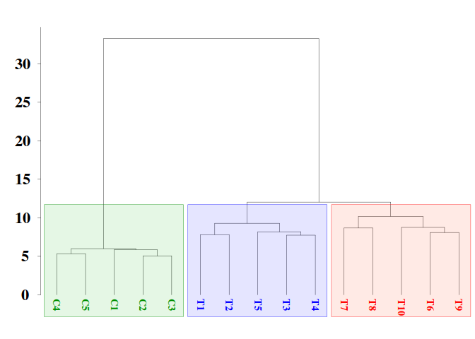
Here, we have use function as.phylo from the R package ape for better dendrogram visualization and function hclust_rect from MethylIT.utils R package to draw rectangles with background colors around the branches of a dendrogram highlighting the corresponding clusters.
5. PCA + LDA
MethylIT function pcaLDA will be used to perform the PCA and PCA + LDA analyses. The function returns a list of two objects: 1) ‘lda’: an object of class ‘lda’ from package ‘MASS’. 2) ‘pca’: an object of class ‘prcomp’ from package ‘stats’. For information on how to use these objects see ?lda and ?prcomp.
Unlike hierarchical clustering (HC), LDA is a supervised machine learning approach. So, we must provide a prior classification of the individuals, which can be derived, for example, from the HC, or from a previous exploratory analysis with PCA.
# A prior classification derived from HC
grps <- cutree(hc, k = 3)
grps[grep(1, grps)] <- "CT"
grps[grep(2, grps)] <- "T1"
grps[grep(3, grps)] <- "T2"
grps <- factor(grps)

ld <- pcaLDA(data = data.frame(dmgm), grouping = grps, n.pc = 3, max.pc = 3,
             scale = FALSE, center = FALSE, tol = 1e-6)
summary(ld$pca)
## Importance of first k=3 (out of 15) components:
## PC1 PC2 PC3
## Standard deviation 41.5183 4.02302 3.73302
## Proportion of Variance 0.9367 0.00879 0.00757
## Cumulative Proportion 0.9367 0.94546 0.95303
We may retain enough components so that the cumulative percent of variance accounted for at least 70 to 80 pca.coord
##           PC1         PC2        PC3
## C1  -21.74024   0.9897934 -1.1708548
## C2  -20.39219  -0.1583025  0.3167283
## C3  -21.19112   0.5833411 -1.1067609
## C4  -21.45676  -1.4534412  0.3025241
## C5  -21.28939   0.4152275  1.0021932
## T1  -42.81810   1.1155640  8.9577860
## T2  -43.57967   1.1712155  2.5135643
## T3  -42.29490   2.5326690 -0.3136530
## T4  -40.51779   0.2819725 -1.1850555
## T5  -44.07040  -2.6172732 -4.2384395
## T6  -50.03354   7.5276969 -3.7333568
## T7  -50.08428 -10.1115700  3.4624095
## T8  -51.07915  -5.4812595 -6.7778593
## T9  -50.27508   2.3463125  3.5371351
## T10 -51.26195   3.5405915 -0.9489265
5.2. Graphic PC1 vs PC2
Next, the graphic for individual coordinates in the two firsts PCs can be easely visualized now:
dt <- data.frame(pca.coord[, 1:2], subgrp = grps)

p0 <- theme(
  axis.text.x  = element_text( face = "bold", size = 18, color="black",
                               # hjust = 0.5, vjust = 0.5,
                               family = "serif", angle = 0,
                               margin = margin(1,0,1,0, unit = "pt" )),
  axis.text.y  = element_text( face = "bold", size = 18, color="black",
                               family = "serif",
                               margin = margin( 0,0.1,0,0, unit = "mm" )),
  axis.title.x = element_text(face = "bold", family = "serif", size = 18,
                              color="black", vjust = 0 ),
  axis.title.y = element_text(face = "bold", family = "serif", size = 18,
                              color="black",
                              margin = margin( 0,2,0,0, unit = "mm" ) ),
  legend.title=element_blank(),
  legend.text = element_text(size = 20, face = "bold", family = "serif"),
  legend.position = c(0.899, 0.12),

  panel.border = element_rect(fill=NA, colour = "black",size=0.07),
  panel.grid.minor = element_line(color= "white",size = 0.2),
  axis.ticks = element_line(size = 0.1), axis.ticks.length = unit(0.5, "mm"),
  plot.margin = unit(c(1,1,0,0), "lines"))

ggplot(dt, aes(x = PC1, y = PC2, colour = grps)) +
  geom_vline(xintercept = 0, color = "white", size = 1) +
  geom_hline(yintercept = 0, color = "white", size = 1) +
  geom_point(size = 6) +
  scale_color_manual(values = c("green4","blue","brown1")) +
  stat_ellipse(aes(x = PC1, y = PC2, fill = subgrp), data = dt, type = "norm",
               geom = "polygon", level = 0.5, alpha=0.2, show.legend = FALSE) +
  scale_fill_manual(values = c("green4","blue","brown1")) + p0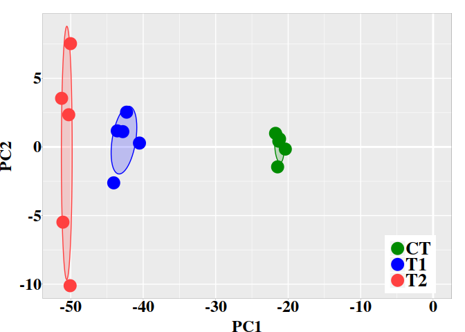
5.3. Graphic LD1 vs LD2
In the current case, better resolution is obtained with the linear discriminant functions, which is based on the three firsts PCs. Notice that the number principal components used the LDA step must be lower than the number of individuals ($N$) divided by 3: $N/3$.
ind.coord <- predict(ld, newdata = data.frame(dmgm), type = "scores")
dt <- data.frame(ind.coord, subgrp = grps)

p0 <- theme(
  axis.text.x  = element_text( face = "bold", size = 18, color="black",
                               # hjust = 0.5, vjust = 0.5,
                               family = "serif", angle = 0,
                               margin = margin(1,0,1,0, unit = "pt" )),
  axis.text.y  = element_text( face = "bold", size = 18, color="black",
                               family = "serif",
                               margin = margin( 0,0.1,0,0, unit = "mm" )),
  axis.title.x = element_text(face = "bold", family = "serif", size = 18,
                              color="black", vjust = 0 ),
  axis.title.y = element_text(face = "bold", family = "serif", size = 18,
                              color="black",
                              margin = margin( 0,2,0,0, unit = "mm" ) ),
  legend.title=element_blank(),
  legend.text = element_text(size = 20, face = "bold", family = "serif"),
  legend.position = c(0.08, 0.12),

  panel.border = element_rect(fill=NA, colour = "black",size=0.07),
  panel.grid.minor = element_line(color= "white",size = 0.2),
  axis.ticks = element_line(size = 0.1), axis.ticks.length = unit(0.5, "mm"),
  plot.margin = unit(c(1,1,0,0), "lines"))

ggplot(dt, aes(x = LD1, y = LD2, colour = grps)) +
  geom_vline(xintercept = 0, color = "white", size = 1) +
  geom_hline(yintercept = 0, color = "white", size = 1) +
  geom_point(size = 6) +
  scale_color_manual(values = c("green4","blue","brown1")) +
  stat_ellipse(aes(x = LD1, y = LD2, fill = subgrp), data = dt, type = "norm",
               geom = "polygon", level = 0.5, alpha=0.2, show.legend = FALSE) +
  scale_fill_manual(values = c("green4","blue","brown1")) + p0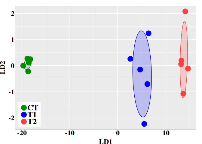
References
- Liese, Friedrich, and Igor Vajda. 2006. “On divergences and informations in statistics and information theory.” IEEE Transactions on Information Theory 52 (10): 4394–4412. doi:10.1109/TIT.2006.881731.
- Stevens, James P. 2009. Applied Multivariate Statistics for the Social Sciences. Fifth Edit. Routledge Academic.