Methylation analysis with Methyl-IT is illustrated on simulated datasets of methylated and unmethylated read counts with relatively high average of methylation levels: 0.15 and 0.286 for control and treatment groups, respectively. The main Methyl-IT downstream analysis is presented alongside the application of Fisher’s exact test. The importance of a signal detection step is shown.
Methyl-IT R package offers a methylome analysis approach based on information thermodynamics (IT) and signal detection. Methyl-IT approach confront detection of differentially methylated cytosine as a signal detection problem. This approach was designed to discriminate methylation regulatory signal from background noise induced by molecular stochastic fluctuations. Methyl-IT R package is not limited to the IT approach but also includes Fisher’s exact test (FT), Root-mean-square statistic (RMST) or Hellinger divergence (HDT) tests. Herein, we will show that a signal detection step is also required for FT, RMST, and HDT as well.
For the current example on methylation analysis with Methyl-IT we will use simulated data. Read count matrices of methylated and unmethylated cytosine are generated with Methyl-IT function simulateCounts. Function simulateCounts randomly generates prior methylation levels using Beta distribution function. The expected mean of methylation levels that we would like to have can be estimated using the auxiliary function:
bmean <- function(alpha, beta) alpha/(alpha + beta)
alpha.ct <- 0.09
alpha.tt <- 0.2
c(control.group = bmean(alpha.ct, 0.5), treatment.group = bmean(alpha.tt, 0.5),
  mean.diff = bmean(alpha.tt, 0.5) - bmean(alpha.ct, 0.5))
## control.group treatment.group mean.diff
## 0.1525424 0.2857143 0.1331719This simple function uses the α and β (shape2) parameters from the Beta distribution function to compute the expected value of methylation levels. In the current case, we expect to have a difference of methylation levels about 0.133 between the control and the treatment.
Methyl-IT function simulateCounts will be used to generate the datasets, which will include three group of samples: reference, control, and treatment.
suppressMessages(library(MethylIT))

# The number of cytosine sites to generate
sites = 50000
# Set a seed for pseudo-random number generation
set.seed(124)
control.nam <- c("C1", "C2", "C3")
treatment.nam <- c("T1", "T2", "T3")

# Reference group
ref0 = simulateCounts(num.samples = 4, sites = sites, alpha = alpha.ct, beta = 0.5,
                      size = 50, theta = 4.5, sample.ids = c("R1", "R2", "R3"))
# Control group
ctrl = simulateCounts(num.samples = 3, sites = sites, alpha = alpha.ct, beta = 0.5,
                      size = 50, theta = 4.5, sample.ids = control.nam)
# Treatment group
treat = simulateCounts(num.samples = 3, sites = sites, alpha = alpha.tt, beta = 0.5,
                       size = 50, theta = 4.5, sample.ids = treatment.nam)
Notice that reference and control groups of samples are not identical but belong to the same population.
The estimation of the divergences of methylation levels is required to proceed with the application of signal detection basic approach. The information divergence is estimated here using the function estimateDivergence. For each cytosine site, methylation levels are estimated according to the formulas: $p_i={n_i}^{mC_j}/({n_i}^{mC_j}+{n_i}^{C_j})$, where ${n_i}^{mC_j}$ and ${n_i}^{C_j}$ are the number of methylated and unmethylated cytosines at site $i$.
If a Bayesian correction of counts is selected in function estimateDivergence, then methylated read counts are modeled by a beta-binomial distribution in a Bayesian framework, which accounts for the biological and sampling variations [1,2,3]. In our case we adopted the Bayesian approach suggested in reference [4] (Chapter 3).
Two types of information divergences are estimated: TV, total variation (TV, absolute value of methylation levels) and Hellinger divergence (H). TV is computed according to the formula: $TV=|p_{tt}-p_{ct}|$ and H:
$H(\hat p_{ij},\hat p_{ir}) = w_i[(\sqrt{\hat p_{ij}} – \sqrt{\hat p_{ir}})^2+(\sqrt{1-\hat p_{ij}} – \sqrt{1-\hat p_{ir}})^2]$ (1)
where $w_i = 2 \frac{m_{ij} m_{ir}}{m_{ij} + m_{ir}}$, $m_{ij} = {n_i}^{mC_j}+{n_i}^{uC_j}+1$, $m_{ir} = {n_i}^{mC_r}+{n_i}^{uC_r}+1$ and $j \in {\{c,t}\}$
The equation for Hellinger divergence is given in reference [5], but
any other information theoretical divergences could be used as well. Divergences are estimated for control and treatment groups in respect to a virtual sample, which is created applying function poolFromGRlist on the reference group.
.
# Reference sample
ref = poolFromGRlist(ref0, stat = "mean", num.cores = 4L, verbose = FALSE)

# Methylation level divergences
DIVs <- estimateDivergence(ref = ref, indiv = c(ctrl, treat), Bayesian = TRUE,
                           num.cores = 6L, percentile = 1, verbose = FALSE)
The mean of methylation levels differences is:
unlist(lapply(DIVs, function(x) mean(mcols(x[, 7])[,1])))## C1 C2 C3 T1 T2
## -0.0009820776 -0.0014922009 -0.0022257725 0.1358867135 0.1359160219
## T3
## 0.1309217360Likewise for any other signal in nature, the analysis of methylation signal requires for the knowledge of its probability distribution. In the current case, the signal is represented in terms of the Hellinger divergence of methylation levels (H).
divs = DIVs[order(names(DIVs))]

# To remove hd == 0 to estimate. The methylation signal only is given for
divs = lapply(divs, function(div) div[ abs(div$hdiv) > 0 ])
names(divs) <- names(DIVs)

# Data frame with the Hellinger divergences from both groups of samples samples
l = c(); for (k in 1:length(divs)) l = c(l, length(divs[[k]]))
data <- data.frame(H = c(abs(divs$C1$hdiv), abs(divs$C2$hdiv), abs(divs$C3$hdiv),
                           abs(divs$T1$hdiv), abs(divs$T2$hdiv), abs(divs$T3$hdiv)),
                   sample = c(rep("C1", l[1]), rep("C2", l[2]), rep("C3", l[3]),
                              rep("T1", l[4]), rep("T2", l[5]), rep("T3", l[6]))
)
Empirical critical values for the probability distribution of H and TV can be obtained using quantile function from the R package stats.
critical.val <- do.call(rbind, lapply(divs, function(x) {
  hd.95 = quantile(x$hdiv, 0.95)
  tv.95 = quantile(x$TV, 0.95)
  return(c(tv = tv.95, hd = hd.95))
}))

critical.val
## tv.95
## C1 0.7893927 81.47256
## C2 0.7870469 80.95873
## C3 0.7950869 81.27145
## T1 0.9261629 113.73798
## T2 0.9240506 114.45228
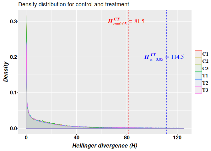
## T3 0.9212163 111.542583.1. Density estimation
The kernel density estimation yields the empirical density shown in the graphics:
suppressMessages(library(ggplot2))

# Some information for graphic
crit.val.ct <- max(critical.val[c("C1", "C2", "C3"), 2]) # 81.5
crit.val.tt <- min(critical.val[c("T1", "T2", "T3"), 2]) # 111.5426

# Density plot with ggplot
ggplot(data, aes(x = H, colour = sample, fill = sample)) +
  geom_density(alpha = 0.05, bw = 0.2, position = "identity", na.rm = TRUE,
               size = 0.4) + xlim(c(0, 125)) +
  xlab(expression(bolditalic("Hellinger divergence (H)"))) +
  ylab(expression(bolditalic("Density"))) +
  ggtitle("Density distribution for control and treatment") +
  geom_vline(xintercept = crit.val.ct, color = "red", linetype = "dashed", size = 0.4) +
  annotate(geom = "text", x = crit.val.ct-2, y = 0.3, size = 5,
           label = 'bolditalic(H[alpha == 0.05]^CT==81.5)',
           family = "serif", color = "red", parse = TRUE) +
  geom_vline(xintercept = crit.val.tt, color = "blue", linetype = "dashed", size = 0.4) +
  annotate(geom = "text", x = crit.val.tt -2, y = 0.2, size = 5,
           label = 'bolditalic(H[alpha == 0.05]^TT==114.5)',
           family = "serif", color = "blue", parse = TRUE) +
  theme(
    axis.text.x  = element_text( face = "bold", size = 12, color="black",
                                 margin = margin(1,0,1,0, unit = "pt" )),
    axis.text.y  = element_text( face = "bold", size = 12, color="black",
                                 margin = margin( 0,0.1,0,0, unit = "mm")),
    axis.title.x = element_text(face = "bold", size = 13,
                                color="black", vjust = 0 ),
    axis.title.y = element_text(face = "bold", size = 13,
                                color="black", vjust = 0 ),
    legend.title = element_blank(),
    legend.margin = margin(c(0.3, 0.3, 0.3, 0.3), unit = 'mm'),
    legend.box.spacing = unit(0.5, "lines"),
    legend.text = element_text(face = "bold", size = 12, family = "serif")
  )
- Hebestreit, Katja, Martin Dugas, and Hans-Ulrich Klein. 2013. “Detection of significantly differentially methylated regions in targeted bisulfite sequencing data.” Bioinformatics (Oxford, England) 29 (13): 1647–53. doi:10.1093/bioinformatics/btt263.
- Hebestreit, Katja, Martin Dugas, and Hans-Ulrich Klein. 2013. “Detection of significantly differentially methylated regions in targeted bisulfite sequencing data.” Bioinformatics (Oxford, England) 29 (13): 1647–53. doi:10.1093/bioinformatics/btt263.
- Dolzhenko, Egor, and Andrew D Smith. 2014. “Using beta-binomial regression for high-precision differential methylation analysis in multifactor whole-genome bisulfite sequencing experiments.” BMC Bioinformatics 15 (1). BioMed Central: 215. doi:10.1186/1471-2105-15-215.
- Baldi, Pierre, and Soren Brunak. 2001. Bioinformatics: the machine learning approach. Second. Cambridge: MIT Press.
- Basu, A., A. Mandal, and L. Pardo. 2010. “Hypothesis testing for two discrete populations based on the Hellinger distance.” Statistics & Probability Letters 80 (3-4). Elsevier B.V.: 206–14. doi:10.1016/j.spl.2009.10.008.
- Sanchez R, Mackenzie SA. Information Thermodynamics of Cytosine DNA Methylation. PLoS One, 2016, 11:e0150427.